Appendix B. Statistical Simulation Studies
B.1 INTRODUCTION
This section presents additional details about the simulation studies used to evaluate the performance of alternative ISM sampling strategies applied to DUs with a range of heterogeneities. Monte Carlo methods were used to collect hypothetical incremental samples following various spatial sampling protocols. The following factors were varied:
- number of increments
- range of variability
- number of replicates
- spatial patterns
- sampling methods
- methods of accounting for compositional and distributional heterogeneities
- sampling patterns
- choice of UCL calculation method
The following performance metrics were used to evaluate the influence of these factors on ISM results:
- coverage of UCL (absolute and relative bias in the estimate of the population mean)
- absolute and/or RPD between the UCL and true mean (SD of relative bias in the population mean)
- RSD of replicate means
The main advantage of simulations is that population parameters are known. Therefore, alternative sampling approaches and calculation methods can be explored for a wide range of scenarios. With each simulation, the same sampling method and/or calculations are performed many times, as if a hypothetical field crew repeated the sampling effort over and over. Because each sampling event involves random sampling from the population, no two hypothetical events yield identical results. However, by repeating the exercise many times, we generate a distribution of results from which we can evaluate the various performance metrics noted above.
Note that not every performance metric is captured in every simulation, in part because the simulations use different approaches to represent bulk material heterogeneity in a DU. Summary tables and discussions of each simulation clarify what metrics were evaluated and how this information can be used to guide the selection of ISM sampling protocols. None of the simulations attempt to explicitly define all seven sources of error in estimates of the mean associated with bulk material sampling (see Section 2.6). The simulations focus on representing the compositional and distributional heterogeneities (CH and DH) that can be attributed to FE and GSE.
Simulations were conducted with defined distributions (statistical or spatial) to represent the variability in sample value results that may be expected, given the combined effect of these errors. Simulations allow for the evaluation of different spatial sampling patterns that cannot be evaluated empirically because the true population parameters (such as population mean) are typically unknown. Naming conventions applied to each simulation experiment include a prefix PD for simulations with probability distributions and M for simulations with maps. The PD simulation approach involved randomly sampling from a two-parameter lognormal PD with a specified mean and variance. The ratio of the population parameters (SD divided by the mean), also known as the CV, provides a measure of variability that facilitates comparisons of results across a wide range of conditions. The M approach involved the use of maps (2D surfaces) to sample from alternative spatial distributions of soil contamination (M). Each set of maps has unique implementations that provide the ability to demonstrate a range of different DU conditions. The method to simulate the soil data for each set of maps follows:
- M-1 is based on a real dataset of more than 200 observations. The sample results were interpolated with inverse distance weighting techniques to yield a completely defined 2D surface of concentrations (see Section B.3).
- M-2 maps are based on real DU data composed of bulk materials. The patterns and concentration values are established from extensive discrete data (100 increments per DU) gathered as a part of multiple ESTCP projects led by Jenkins and Hewitt (Jenkins et al. 2004, Hewitt et al. 2005) (Jenkins et al. 2004, Hewitt et al. 2005); and Qiao, Pulsipher, and Hathaway (Qiao et al. 2010) (Qiao et al. 2010) document the specific details for how the discrete data were used to establish the completely defined 2D surface of increment values shown Section B.4.
Collectively, the simulation studies presented in this appendix provide a preliminary set of results intended to facilitate the development of ISM sampling designs and corresponding statistical analyses. More detail and underlying assumptions of the different simulation approaches are identified below.
Simulations presented in this appendix refer to different scales of heterogeneity as being “small” and “large,” and are not intended to imply a precise dimension for a DU in terms of acres. Instead, the terms are relative to the size of the DU. Small scale refers to the immediate vicinity of the incremental sample, whereas large scale refers to the overall spatial extent of the DU.
B.1.1 Summary of Simulation Findings
Table B-1 summarizes the observations and conclusions from the various statistical simulations that were conducted.
Table B-1. Summary of findings from simulation experiments using PDs (PD) and maps (M).
Source: 2012, ITRC ISM Team.
| Effects of the Number of Increments and Replicates on the Estimate of the Mean | |
| 1 | Increasing the number of increments and/or replicates reduces variability in the estimate of the mean. |
| 2 | Variability in the grand mean (the mean of the replicate incremental sampling estimates of the mean) is a function of the total number of increments collected (increments x replicates). |
| 3 | DUs with high heterogeneous contaminant concentrations have greater variability in the estimate of the mean and greater potential for errors in terms of both frequency and magnitude. Underestimates of the mean would be expected to occur more frequently than overestimates for heterogeneous sites with right-skewed contaminant concentration distributions. With equal numbers of samples (that is, individual discrete samples versus ISM replicates), the magnitude of error in estimating the mean would be expected to be lower using ISM. |
| 4 | The coverage of the 95% UCL depends on the total sample size (increments × replicates). For the typical number of increments of an ISM sampling design (30 to 100), increasing the number of ISM replicates above three provides marginal return in terms of improving coverage, but increasing the number of replicates decreases (or improves) the RPD, meaning that it will produce estimates of the 95% UCL closer to the DU mean. |
| 5 | Simulations produced varying results in terms of improvement in coverage by increasing the number of increments. As with increasing replicates, increasing the number of increments decreases (i.e., improves) the RPD. |
| 6 | Coverage provided by the two UCL calculation methods depends on the degree of variability of the contaminant distribution within the DU. For DUs with medium or high heterogeneity, the Student’s-t method may not provide specified coverage. For DUs with high heterogeneity, the Chebyshev method may not provide specified coverage as well. |
| 7 | The Chebyshev method always provides a higher 95% UCL than the Student’s-t method for a given set of ISM data with r > 2. When both methods provide specified coverage, the Chebyshev consistently yielded a higher RPD. |
| Effects of Sampling Pattern | |
| 8 | If the site is relatively homogeneous, all three field sampling patterns yield unbiased mean estimates, but the magnitude of error in the mean may be higher with simple random sampling compared to systematic random sampling. All sampling patterns yield similar coverages. |
| 9 | While all three sampling options are statistically defensible, collecting increments within the DU using simple random sampling is most likely to generate an unbiased estimate of the mean and variance according to statistical theory. From a practical standpoint, true random sampling is probably the most difficult to implement in the field and may leave large parts of the DU “uncovered,” or without any increment sample locations. It should be noted that random does not mean wherever the sampling team feels like taking a sample, and a formal approach (typically based on a random number generator) to determining the random sample locations must be used. |
| 10 | Systematic random sampling can avoid the appearance that areas are not adequately represented in ISM samples and is relatively straightforward to implement in the field. Theoretically, it is inferior to simple random sampling for obtaining unbiased samples and can be more prone to producing errors in estimating the true mean, especially if the contamination is distributed in a systematic way. Random sampling within a grid is, in a sense, a compromise approach, with elements of both simple random and systematic sampling. |
| Subdividing the DU | |
| 11 | Sampling designs with this method yield unbiased estimates of the mean. |
| 12 | The principal advantage of subdividing the DU is that some information on heterogeneity in contaminant concentrations across the DU is obtained. If the DU fails the decision criterion (that is, it has a mean or 95% UCL concentration above a soil action limit), information will be available to indicate whether the problem exists across the DU or is confined to guide redesignation of the DU and resampling to further delineate areas of elevated concentrations. |
| 13 | Partitioned DU SE estimates are larger than those from replicate data if the site is not homogeneous. Hence, 95% UCL estimates from a subdivided DU will be as high or higher than those obtained from replicate measurements collected across the DU. The higher 95% UCLs improve coverage (generally attain 95% UCL) and increase the RPD. These increases occur if unknown spatial contaminant patterns are correlated with the partitions. In most cases, the Student’s-t method provides adequate coverage. |
| RSD | |
| 14 | Datasets with a high RSD are more likely to achieve specified coverage for 95% UCL than datasets with low RSD. This tendency is explained by the greater variability among replicates leading to higher 95% UCL values, resulting in better coverage. |
| 15 | A low RSD does not ensure specified coverage by the 95% UCL or low bias in a single estimate of the mean. The opposite is, in fact, the case. For situations in which the UCL or one replicate mean is less than the true mean, the underestimate increases as RSD decreases. |
The simulation findings presented in this appendix do not represent the totality of simulation exercises conducted as part of this project. It is anticipated that additional research may be needed to further investigate the performance of alternative ISM sample designs.
B.2 Probability Distributions (PDs)
A series of Monte Carlo simulations was run using PDs with different CVs. Table B-2 summarizes distribution variability (based on CV) and results for selected sampling designs and performance metrics (both Student’s-t and Chebyshev UCLs).
Each scenario can be thought of as a special case of the simulations with maps (M-1 and M-2), presented later in this appendix. With sampling from PDs, each increment is an independent random sample obtained from the same defined distribution (that is, they are identically distributed), which is analogous to using simple random sampling for increment collection for an actual site. The DU is assumed to consist of a single population of lognormally distributed concentrations. It is important to note that, while this approach is useful for conveying important concepts about ISM, sampling from a PD is an oversimplification for the following reasons:
- There is no attempt to quantify the relative contributions of different sources of heterogeneity or errors introduced in both the field and laboratory. The variance is viewed as a lumping term that represents the variability in concentrations in soil if the site were divided into samples of some mass. In practice, the expected error in the estimate of the mean depends in part on the mass of soil collected with each increment (see discussion of Gy’s sampling principles in Section 2.6). Therefore, it is convenient to think of the population as having a fixed mean concentration but also a variance contingent on the sample mass. The simulations with defined distributions do not explore the effect of sample mass on performance metrics. Instead, it is assumed that the specified variance simply reflects the collective sources of heterogeneity.
- The defined populations used in the simulations are not described as representing a DU of a specific size. At many sites, it is common for concentrations to exhibit spatial patterns, including subareas of elevated concentrations and overlapping sources (that is, mixtures). This may be true even for very small DUs where concentrations from samples collected within a 1-ft radius differ by more than an order of magnitude. Most of the simulations do not explicitly model these conditions but instead presume that the overall population for the DU can be approximated by a lognormal distribution, regardless of any spatial arrangement of the contaminant mass.
- Only lognormal PDs are defined, and alternative positively skewed PDs were not explored. In general, because lognormal distributions give greater weight to results in the upper tail than alternative choices (for example, gamma or Weibull distribution), the SE for the mean and the corresponding UCLs tends be higher than that of comparable distributions with the same population mean and variance.
Table B-2. Summary of simulation results using lognormal distributions (* %itl = percentile).
Source: 2012, ITRC ISM Team.
95% UCL >= true mean [overestimate of mean]
| Statistic* | Chebyshev 95% UCL | Student’s-t 95% UCL | ||||||
| 2 reps | 3 reps | 5 reps | 7 reps | 2 reps | 3 reps | 5 reps | 7 reps | |
| m=30, CV=1 | ||||||||
| count of simulations | 4,571 | 4,835 | 4,956 | 4,981 | 4,693 | 4,664 | 4,689 | |
| 95% UCL coverage | 91% | 97% | 99% | 100% | 94% | 93% | 94% | 94% |
| mean RPD | 27% | 22% | 18% | 16% | 37% | 16% | 10% | 8% |
| 5th %ile RPD | 3% | 4% | 5% | 5% | 4% | 2% | 1% | 1% |
| 50th %ile RPD | 22% | 21% | 17% | 15% | 31% | 14% | 9% | 7% |
| 95th %ile RPD | 65% | 48% | 34% | 28% | 91% | 34% | 20% | 15% |
| m=30, CV=4 | ||||||||
| count of simulations | 4,346 | 4,690 | 4,852 | 4,909 | 4,519 | 4,430 | 4,333 | 4,351 |
| 95% UCL coverage | 87% | 94% | 97% | 98% | 90% | 89% | 87% | 87% |
| mean RPD | 93% | 80% | 63% | 55% | 129% | 57% | 36% | 28% |
| 5th %ile RPD | 6% | 8% | 9% | 10% | 9% | 4% | 3% | 2% |
| 50th %ile RPD | 65% | 59% | 50% | 44% | 90% | 41% | 27% | 22% |
| 95th %ile RPD | 272% | 214% | 155% | 129% | 374% | 157% | 92% | 73% |
| m=30, CV=7 | ||||||||
| count of simulations | 4,171 | 4,532 | 4,740 | 4,820 | 4,414 | 4,187 | 4,101 | 4,137 |
| 95% UCL coverage | 83% | 91% | 95% | 96% | 88% | 84% | 82% | 83% |
| mean RPD | 140% | 117% | 94% | 83% | 189% | 86% | 55% | 45% |
| 5th %ile RPD | 8% | 8% | 9% | 11% | 11% | 5% | 4% | 3% |
| 50th %ile RPD | 82% | 73% | 65% | 59% | 111% | 54% | 36% | 30% |
| 95th %ile RPD | 457% | 358% | 271% | 227% | 609% | 272% | 164% | 133% |
| m=100, CV=1 | ||||||||
| count of simulations | 4,604 | 4,827 | 4,946 | 4,979 | 4,720 | 4,690 | 4,687 | 4,669 |
| 95% UCL coverage | 92% | 97% | 99% | 100% | 94% | 94% | 94% | 93% |
| mean RPD | 27% | 23% | 18% | 16% | 38% | 16% | 10% | 8% |
| 5th %ile RPD | 3% | 5% | 5% | 5% | 4% | 3% | 2% | 1% |
| 50th %ile RPD | 22% | 21% | 18% | 15% | 32% | 14% | 9% | 7% |
| 95th %ile RPD | 66% | 49% | 34% | 28% | 93% | 35% | 20% | 15% |
| m=100, CV=4 | ||||||||
| count of simulations | 4,358 | 4,674 | 4,858 | 4,926 | 4,547 | 4,435 | 4,375 | 4,395 |
| 95% UCL coverage | 87% | 93% | 97% | 99% | 91% | 89% | 88% | 88% |
| mean RPD | 95% | 79% | 64% | 55% | 130% | 57% | 36% | 28% |
| 5th %ile RPD | 6% | 9% | 10% | 10% | 9% | 5% | 3% | 2% |
| 50th %ile RPD | 65% | 59% | 51% | 45% | 89% | 41% | 27% | 22% |
| 95th %ile RPD | 280% | 211% | 157% | 129% | 380% | 155% | 95% | 73% |
| m=100, CV=7 | ||||||||
| count of simulations | 4,115 | 4,509 | 4,739 | 4,839 | 4,362 | 4,186 | 4,092 | 4,119 |
| 95% UCL coverage | 82% | 90% | 95% | 97% | 87% | 84% | 82% | 82% |
| mean RPD | 135% | 114% | 93% | 80% | 183% | 84% | 54% | 43% |
| 5th %ile RPD | 7% | 8% | 9% | 9% | 10% | 5% | 3% | 3% |
| 50th %ile RPD | 82% | 74% | 64% | 58% | 111% | 53% | 36% | 30% |
| 95th %ile RPD | 417% | 321% | 251% | 210% | 557% | 240% | 156% | 122% |
| Chebyshev 95% UCL | Student’s-t 95% UCL | ||||||
| 2 reps | 3 reps | 5 reps | 7 reps | 2 reps | 3 reps | 5 reps | 7 reps |
| m=30, CV=1 | |||||||
| 4,678429 | 165 | 44 | 19 | 307 | 336 | 311 | 322 |
| 91% | 97% | 99% | 100% | 94% | 93% | 94% | 94% |
| -4% | -3% | -2% | -1% | -4% | -3% | -2% | -2% |
| -11% | -7% | -7% | -3% | -11% | -8% | -6% | -5% |
| -4% | -2% | -1% | -1% | -4% | -2% | -2% | -1% |
| 0% | 0% | 0% | 0% | 0% | 0% | 0% | 0% |
| m=30, CV=4 | |||||||
| 654 | 310 | 148 | 91 | 481 | 570 | 667 | 649 |
| 87% | 94% | 97% | 98% | 90% | 89% | 87% | 87% |
| -13% | -10% | -7% | -6% | -13% | -10% | -8% | -6% |
| -30% | -23% | -18% | -15% | -30% | -25% | -19% | -17% |
| -12% | -8% | -6% | -5% | -11% | -8% | -6% | -5% |
| -1% | -1% | 0% | 0% | -1% | -1% | -1% | -1% |
| m=30, CV=7 | |||||||
| 829 | 468 | 260 | 180 | 586 | 813 | 899 | 863 |
| 83% | 91% | 95% | 96% | 88% | 84% | 82% | 83% |
| -18% | -13% | -10% | -8% | -18% | -14% | -11% | -9% |
| -39% | -31% | -24% | -21% | -41% | -32% | -28% | -23% |
| -16% | -11% | -8% | -6% | -16% | -12% | -9% | -8% |
| -2% | -1% | 0% | -1% | -1% | -1% | -1% | -1% |
| m=100, CV=1 | |||||||
| 396 | 173 | 54 | 21 | 280 | 310 | 313 | 331 |
| 92% | 97% | 99% | 100% | 94% | 94% | 94% | 93% |
| -4% | -3% | -2% | -1% | -5% | -3% | -2% | -2% |
| -12% | -8% | -5% | -3% | -12% | -9% | -6% | -5% |
| -3% | -2% | -2% | -1% | -4% | -3% | -2% | -1% |
| 0% | 0% | 0% | 0% | 0% | 0% | 0% | 0% |
| m=100, CV=4 | |||||||
| 642 | 326 | 142 | 74 | 453 | 565 | 625 | 605 |
| 87% | 93% | 97% | 99% | 91% | 89% | 88% | 88% |
| -13% | -10% | -6% | -6% | -13% | -10% | -7% | -6% |
| -30% | -23% | -18% | -18% | -31% | -25% | -18% | -16% |
| -11% | -8% | -5% | -5% | -12% | -9% | -6% | -5% |
| -1% | -1% | 0% | 0% | -1% | -1% | 0% | 0% |
| m=100, CV=7 | |||||||
| 885 | 491 | 261 | 161 | 638 | 814 | 908 | 881 |
| 82% | 90% | 95% | 97% | 87% | 84% | 82% | 82% |
| -17% | -13% | -9% | -8% | -17% | -14% | -11% | -9% |
| -39% | -29% | -22% | -20% | -38% | -31% | -26% | -23% |
| -15% | -11% | -8% | -6% | -15% | -12% | -9% | -8% |
| -1% | -1% | -1% | -1% | -1% | -1% | -1% | -1% |
B.2.1 Methods
Monte Carlo analysis was used to repeatedly apply a specified sampling design (number of increments and ISM samples) to a DU scenario. Typically, between 5,000 and 30,000 trials were used, with the large number of trials expected to yield relatively stable (that is, reproducible) results. Each trial represents a complete sampling event (n increments and r replicates) and yields an estimate of the population mean, the SE of the mean, and the 95% UCL. Collectively, the results yield a distribution of 95% UCLs that can be used to calculate performance metrics – for example, ideally, the sampling method and UCL calculation yield a PD of 95% UCLs with a 5th percentile equal to (or greater than) the true population mean. This would mean that we can expect the sampling design applied to this type of population to achieve the desired coverage (or percentage of exceedances of the true mean) of 95%. Table B-2 provides examples of simulation experiments with coverages that vary from approximately 80 to 100%.
Multiple ISM samples (or replicates) must be collected to calculate the SE and UCL. The expected small sample sizes (three to seven replicates) for most implementations of ISM preclude the use of bootstrap resampling techniques to calculate a UCL, so simulations were performed using only the Student’s-t and Cheybshev UCL methods, which are based on sample size, sample mean, and variance. Because the distribution of sample means tends to exhibit less skew than the population due to the CLT, the performance of the Student’s-t UCL can vary, but Student’s-t can be expected to yield the most reliable performance metrics for populations with a low (≤1) CV. By contrast, Chebyshev generally yields higher UCLs with higher coverage but also higher RPDs. RPD = [(UCL – μ)/100] ´ 100%, where μ denotes the true DU (population) mean.
Generally, sampling designs were varied between 15 and 100 increments and between two and seven replicate ISM samples. The mean of the distribution represents the population mean and is used to calculate the bias and RPD metrics.
The number of replicates is used to represent the degrees of freedom in UCL calculations using ISM.
B.2.2. Results
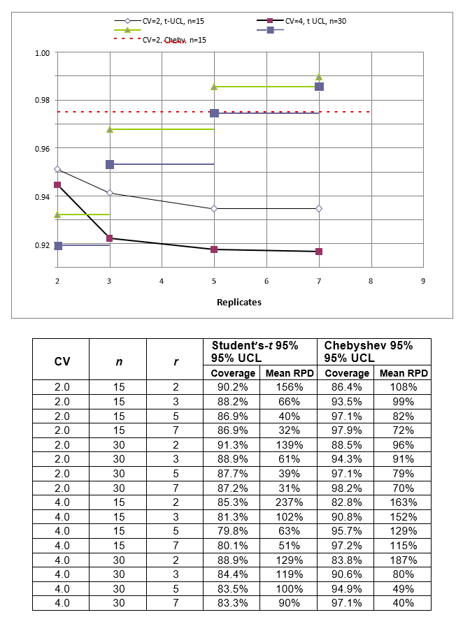
Figure B-1 illustrates how the coverage of the 95% UCL varies for the Student’s-t and Chebyshev UCL equations for a range of sampling designs applied to lognormal distributions with a range of variability. The table below the graph gives the coverage statistics as well as the average RPD (based on the full distribution of UCLs calculated).
Source: 2012, ITRC ISM Team.
These examples are useful for illustrating the following general patterns that emerge from the simulation experiments with lognormal distributions:
- The Chebyshev UCL generally yields higher coverage than the Student’s-t UCL, with the exception of scenarios in which two replicates (r = 2) are selected. The upper critical value of the Student’s-t distribution (that is, the t-value) varies with the degrees of freedom (df = r – 1), as noted below. For r = 2, the t-value is 6.3, which introduces an additional factor of two or more to the calculation of the 95% UCL compared to sampling designs with three or more replicates.
Table B-3. 95th Percentiles of Student’s t Distribution
Source: 2020, ITRC ISM Update Team.
| Replicates | df = r – 1 | t-value for alpha = 0.05 |
| 2 | 1 | 6.3 |
| 3 | 2 | 2.9 |
| 4 | 3 | 2.4 |
| 5 | 4 | 2.1 |
| 6 | 5 | 2.0 |
| 7 | 6 | 1.9 |
- The coverage of the Chebyshev UCL generally increases with increasing sample sizes (increments and replicates) but with diminishing returns. The table below lists examples of combination of replicates and increments that can be expected to yield approximately 95% coverage. The coverage of the Student’s-t UCL generally does not achieve 95% and does not increase with increasing samples sizes (increments and replicates) within a practical range.
Table B-4. Coverage of the Chebyshev UCL
Source: 2020, ITRC ISM Update Team.
| CV | Increments | Replicates | Coverage | CV | Increments | Replicates | Coverage |
| 1 | 15 | 3 | 96% | 4 | 30 | 4 | 94% |
| 30 | 3 | 97% | 50 | 4 | 95% | ||
| 2 | 15 | 3 | 93% | 100 | 3 | 93% | |
| 15 | 4 | 95% | 100 | 4 | 96% | ||
| 30 | 3 | 94% | 7 | 30 | 5 | 95% | |
| 30 | 4 | 96% | 100 | 5 | 95% | ||
| 3 | 15 | 5 | 95% | ||||
| 30 | 4 | 95% | |||||
| 50 | 4 | 96% | |||||
| 100 | 3 | 95% |
- The RPD between the 95% UCL and the population mean is generally greater for Chebyshev than Student’s-t, particularly for trials in which the 95% UCL actually exceeds the population mean. Therefore, the trade-off with the Chebyshev UCL is that it achieves more reliable coverage but also higher UCLs.
- The simulations with lognormal distributions yield unbiased estimates of the mean.
B.3 SPATIAL AUTOCORRELATION MAPS (M-1)
For most sites, contaminants in soil exhibit some degree of spatial relationship, meaning that variance in the concentration often reduces as the distance between sample locations decreases. It is well established that strong spatial relationships can reduce the effective sample size of a dataset because each sample provides some redundant information (Cressie 1993). In statistical terms, this redundancy violates the assumption that observations are independent. ISM CIs generated from spatially related data can be too narrow, resulting in a higher frequency of decision errors. Spatial relationships may also introduce bias in estimates of the mean and variance, depending on the sampling protocol. Bias can be reduced by using a truly random sampling strategy (for example, simple random sampling). The issue of spatial relationships applies to discrete as well as ISM sampling.
B.3.1. Methods
Simulations were run to evaluate the effect of spatial autocorrelation on the performance of ISM. Figure B-2 shows a map generated from a real dataset of more than 200 observations. The sample results were interpolated with inverse distance weighting techniques to yield a 2D surface of concentrations. Such spatial smoothing is likely to underestimate the distributional heterogeneity in concentrations that exists at most sites, so the results with ISM may underestimate the variance. Four ISM sampling protocols were applied to this map, assuming the map represents a single DU:
- systematic grid with a random start location (no division of the DU)
- systematic grid with a random start location (division of DU into quadrants)
- simple random sample (no division of the DU)
- simple random sample (division of the DU into quadrants)
For the scenario in which the site is divided into quadrants, each quadrant was sampled with the specified number of replicates, which means simulations with quadrants represent an overall fourfold increase in the sampling effort. Alternative evaluations of the quadrant scenario were evaluated with different maps to illustrate the performance metrics for quadrants in which a single ISM sample is collected from each quadrant, yielding a total sample size of r = 4.
B.3.2. Results
Table B-3 summarizes the simulation results with 1,000 Monte Carlo trials using 30 increments and three, five, and seven replicates. The distribution is only mildly skewed (CV = 0.7), and the autocorrelation is high (Moran’s I z-score = 3.8). The following observations are noted:
- The spatial autocorrelation does not affect the coverage of either the simple random sampling or systematic grid sampling. With 30 increments and three replicates, Chebyshev yields 96 to 97% coverage, whereas Student’s-t yields 94% coverage.
- As noted with the simulations using lognormal distributions, increasing the number of replicates results in a higher coverage for the Chebyshev UCL but generally no improvement in the Student’s-t UCL.
- The average RPD for the 95% UCL is lower by approximately a factor of two with systematic grid sampling, but introducing spatial autocorrelation tends to result in an improvement in this metric, most likely because autocorrelation affects the correlation between the sample mean and variance. For non-normal distributions, simple random sampling yields a positive correlation between the sample mean and sample variance. When systematic grid sampling is applied to a scenario with high spatial autocorrelation, it is more likely that neighboring samples share similar values, thereby reducing the sample variance.
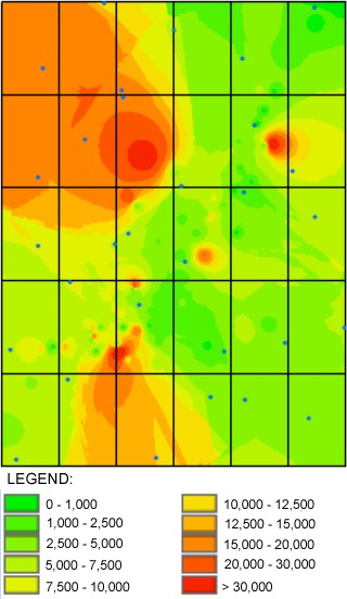
Source: Kelly Black, Neptune and Company, Inc., 2012. Used with permission.
- Throughout the entire DU (all grid cells combined), the population mean is 8,564 and SD is 6,507 (CV = 0.7).
Table B-5. Summary of simulation results for a site with high spatial autocorrelation (see map in Figure B-2).
Source: Kelly Black, Neptune and Company, Inc., 2012. Used with permission.
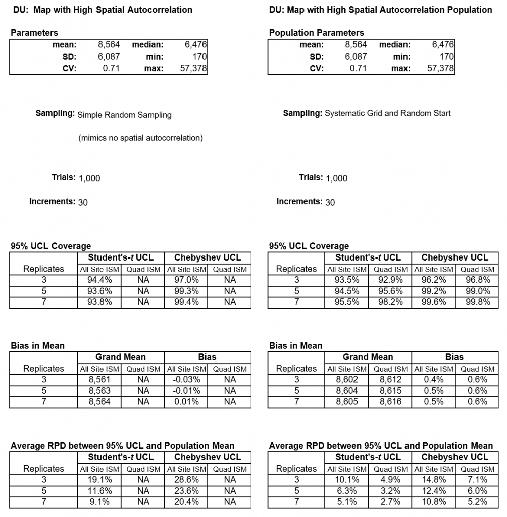
- Both sampling protocols yield relatively unbiased estimates in the mean, which is an expected result for simple random sampling but not necessarily for systematic grid sampling. However, even for a site with high spatial autocorrelation, the bias is negligible when the population has a very low CV.
- Splitting the DU into quadrants results in lower RPDs, mainly reflecting the increase in the total number of replicates.
B.4. MAPS OF RDX AND HMX (M-2A AND M2-B)
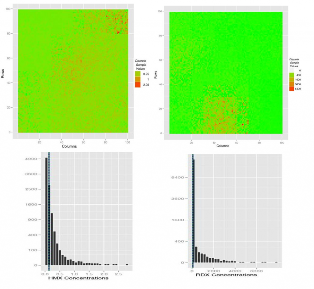
Map scenarios M-2A and M-2B represent different spatial structures with both small- and large-scale distributional heterogeneities. These examples are based on a more extensive analysis of ISM conducted for USACE and discussed in a separate report (Qiao et al. 2010). The data are based on results of site investigations involving measurements of concentrations of RDX and HMX in (discrete) bulk surface soil samples. The two histograms in Figure B-3 show each of these sites in 2D histograms with a square-root-transformed count axis to improve the visualization of the tail values. With a standard count axis shown, these distributions would look even more extreme. Their respective means are marked with a dotted green vertical line.
The plots on the left represent a distribution of HMX (mg/kg), and the plots on the right site represent a distribution of RDX (mg/kg) from which increments will be collected. Obstructions such as large rocks and paved roads are excluded to simplify the automation of ISM sampling as well as to simplify the calculation of the population parameter (true mean) from which performance metrics are determined.
Source: J. Hathaway for ACOE, 2012. Used with permission.
B.4.1 Descriptions of DUs
Qiao, Pulsipher, and Hathaway (Qiao et al. 2010) provide details about how the simulated sites were created and values were applied to grid cells representing the DUs. Briefly, each of the 10,000 discrete increment concentration values shown on each site in Figure B-3 are derived from real sites composed of bulk materials. The patterns and concentration values are from extensive discrete data (increments) gathered as a part of multiple ESTCP projects led by Jenkins and Hewitt (Jenkins et al. 2004). Each grid value (increment) in Figure B-3 represents the agglomeration of the bulk material from that area with reported values of constituent levels in units of mg per kg (or parts per million). Thus, as with the simulations with lognormal distributions (PD-1), FE and GSE were not explicitly used in simulating these sites. These errors are implicitly accounted for in the modeled small-scale (local) spatial variability.
B.4.1.1. HMX DU (M2-A)
The HMX concentrations (mg/kg) shown in Figure B-3 (map and histogram on left) depict a 10-m × 10-m DU with moderate heterogeneity. This DU has some spatial patterns, but they are relatively dispersed, and the distribution of values is relatively tight (CV = 1.1). Population parameters include a (true) mean of 0.13, an SD of 0.15, and a maximum of approximately 2.3 mg/kg.
B.4.1.2. RDX DU (M2-B)
The RDX concentrations (mg/kg) shown in Figure B-3 (map and histogram on the right) depict a 10-m × 10-m DU with more extreme heterogeneity. The map shows one area with extremely high concentrations (bottom middle) and a second area with high concentrations (middle right side) while the rest of the DU has orders of magnitude lower concentrations. This DU represents a site with relatively strong small- and large-scale distributional heterogeneity with a CV of approximately 4.5 (SD = 319 mg/kg; mean = 71.4 mg/kg).
B.4.2 ISM sampling patterns
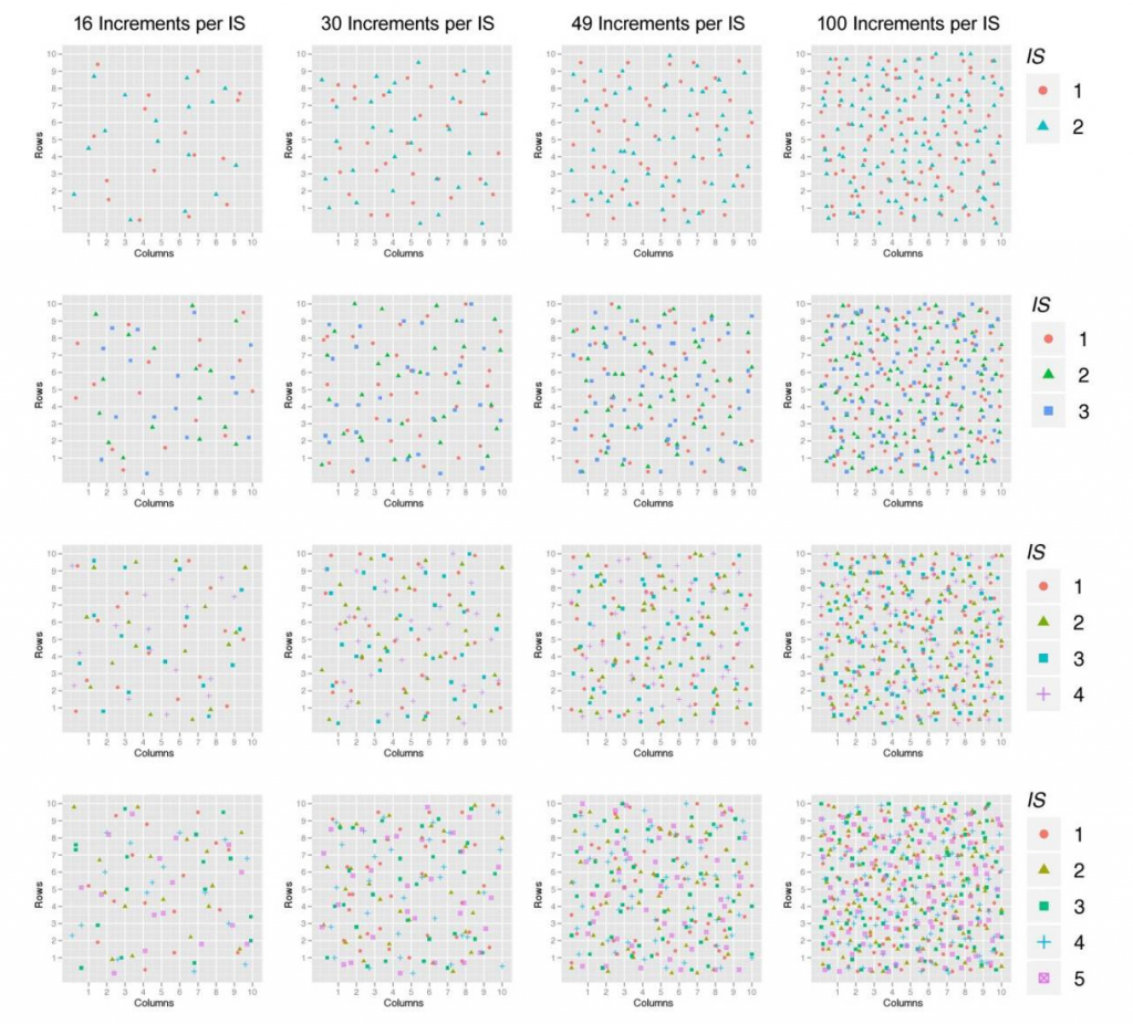
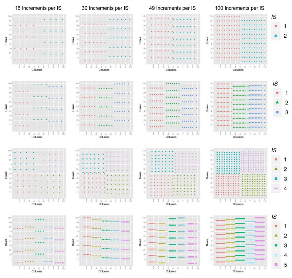
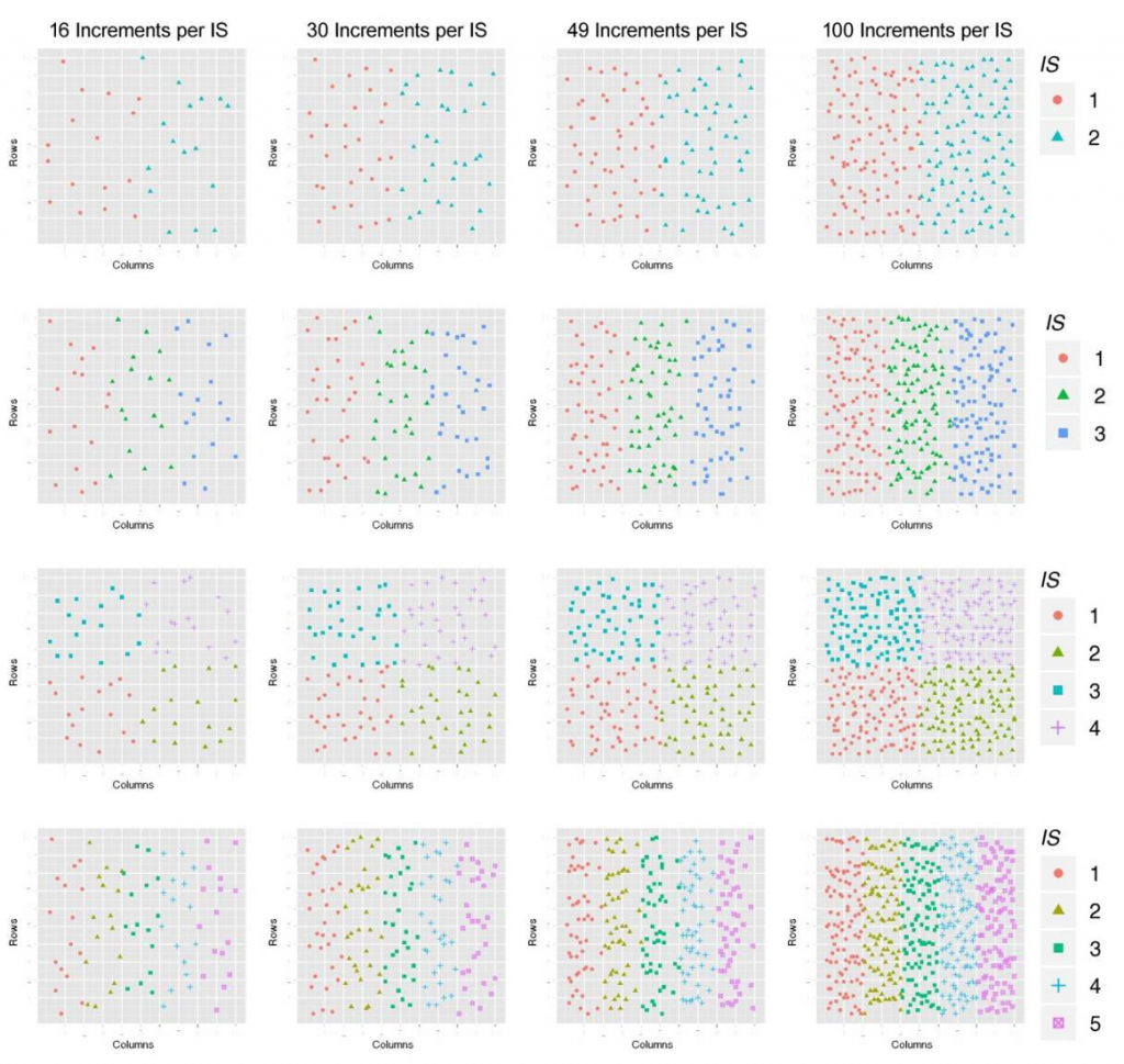
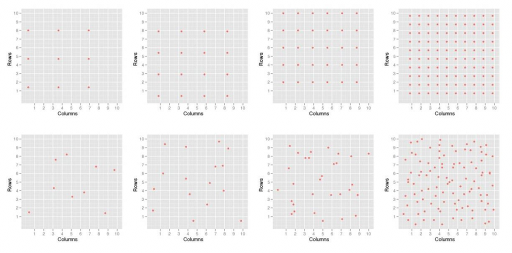
Figures B-4 to B-7 show the 64 different ISM patterns that are evaluated and summarized in Section B.4.4. For all four figures, each row of plots represents a different number of replicates gathered from the DU (two, three, four, and five), and each column of plots identifies a different number of increments per replicate (16, 30, 49, and 100). Figure B-4 and Figure B-5 show the standard ISM procedure with replicate ISMs over the entire DU for systematic and random grid sampling, respectively. Figure B-6 and Figure B-7 represent the grouped ISM methods for systematic and random grid sampling, respectively. In particular, they show the general structure for each of the evaluated patterns but represent only an example of one random selection for each pattern. Figure B-8 shows the random and systematic discrete sampling types that were evaluated using sample sizes of 9, 16, 30, and 100. Once again, these examples show the general structure for each of the evaluated sampling types and only represent one random selection for each pattern.

Source: J. Hathaway for ACOE, 2012. Used with permission.
Source: J. Hathaway for ACOE, 2012. Used with permission.
Source: J. Hathaway for ACOE, 2012. Used with permission.
Source: J. Hathaway for ACOE, 2012. Used with permission.
Source: J. Hathaway for ACOE, 2012. Used with permission.
B.4.3 Results using discrete sampling
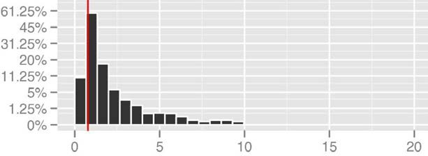
Table B-4 shows a few of the 2,000 iterations from the UCL calculations based on using the mean and SE calculated from nine systematic grid discrete samples (see upper left plot in Figure A-8) from a DU. These values represent absolute concentrations in mg/kg, and the values from the UCL column are then compared to the true mean. A sampling design achieves the desired statistical coverage if, for example, the UCL values underestimate the true mean in fewer than 100 of the 2,000 iterations (that is, 5%). Figure B-9 shows a histogram of 2,000 UCL values from one simulation scenario where the y-axis represents the percentage of 2,000 in each bin (note that the y-axis is distorted to show the low bin counts). The red line identifies the location of the true mean. This UCL histogram shows that the coverage was only 76%, which is a significant departure from the theoretical design of 95% UCL. The simulation results provide an example demonstrating how one of the performance metrics (coverage of the 95% UCL) may indicate whether a particular sampling design is unlikely to yield reliable results.
Table B-6. Example of mean and 95% UCL calculations for each iteration of a simulation.
Source: J. Hathaway for ACOE, 2012. Used with permission.
| Mean | UCL |
| 0.61 | 0.76 |
| 0.72 | 0.94 |
| 1.01 | 1.46 |
| 0.79 | 1.18 |
| … | … |
| 0.81 | 1.02 |
Source: J. Hathaway for ACOE, 2012. Used with permission.
For display purposes, the y-axis in Figure B-9 is in terms of percentage of 2,000 and is distorted (not evenly spaced between ticks) to highlight the low count bins. The red line identifies the true mean of 0.776.
The discrete sampling examples were restricted to calculations using Student’s-t UCL and Chebyshev UCLs. Other methods for UCL calculations are typically considered to attain appropriate coverage by implementing USEPA’s ProUCL or comparable software. For sites with heavy right-tailed distributions and distributional heterogeneity, discrete sampling methods with up to 100 samples taken are not sufficient to use a t-statistic to calculate a reliable UCL. However, the Chebyshev UCL does provide adequate coverage for many of the DUs at multiple sample sizes. Additional discrete sampling results are discussed in the subsequent sections.
B.4.4. Results using ISM
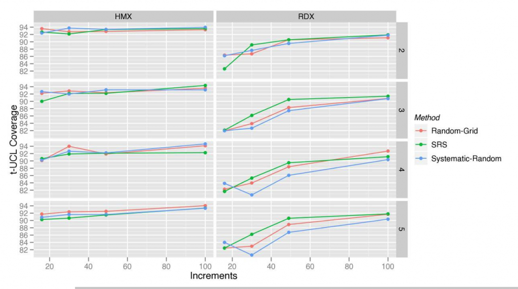
The following subsections provide results for the RDX and HMX DUs. Within each simulated DU subsection, 40 sets of results are shown using two different UCL calculation methods. Both systematic grid and random grid sampling routines for the grouped and standard ISM patterns were used. Differences in results for these sampling routines were within the range of simulation (stochastic) error. Figure B-10 shows an example of the equal coverage for both M2-A and M2-B using the three different standard ISM sample selection patterns (random grid, simple random, and systematic random) for t-based 95% UCLs. For simplicity, only the results associated with the random grid sampling routines are presented in each section.
The tables shown in each section will be separated into the three general sampling patterns: standard ISM, grouped ISM, and discrete sampling. Each table summarizes the results from 2,000 iterations, but the first two columns are different for the ISM and discrete summary tables. For the ISM summary tables, the first column identifies the number of ISMs sampled from within the DU, and the second column shows the number of increments in each ISM. For the discrete summary tables, the first column identifies whether random or systematic sampling was used, and the second column lists the number of increments sampled from the DU that are used to calculate the mean and SD. The third and fourth columns show the UCL coverage for the Chebyshev and t-UCL calculations. The last four columns summarize the RPD of the UCL values using the Chebyshev and t-distribution UCL multipliers. The RPD above column for each UCL multiplier is the average relative difference from the true mean for those UCL values that were above the true mean. The RPD below columns for each UCL multiplier show the average relative difference from the true mean for those UCL values that were below the true mean.
Source: J. Hathaway for ACOE, 2012. Used with permission.
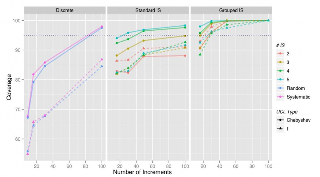
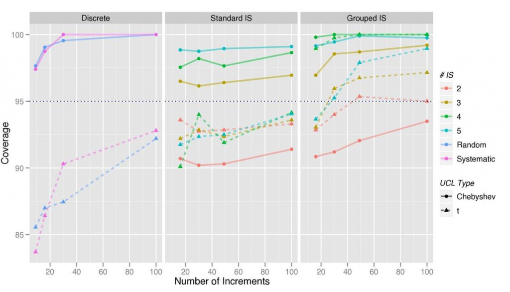
Each subsection contains plots depicting the pertinent information from the coverage tables for an easier visualization of the results from simulation studies. These plots show the designed UCL coverage level (dashed blue line) and the coverage performance of each sampling pattern as a function of the number of increments (in each ISM for the ISM designs and total for discrete designs). Each colored line represents a different sampling pattern with a separate plot for the discrete, grouped ISM, and standard ISM. The dashed line identifies the t-UCL calculations, and the solid line identifies the Chebyshev UCL values. Each plotted point represents the results from one line from the tables within the subsection. Coverage results based on 2000 iterations provide estimates accurate to within approximately ±1.5% to ±2.5%.
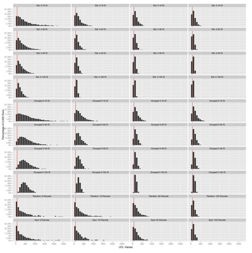
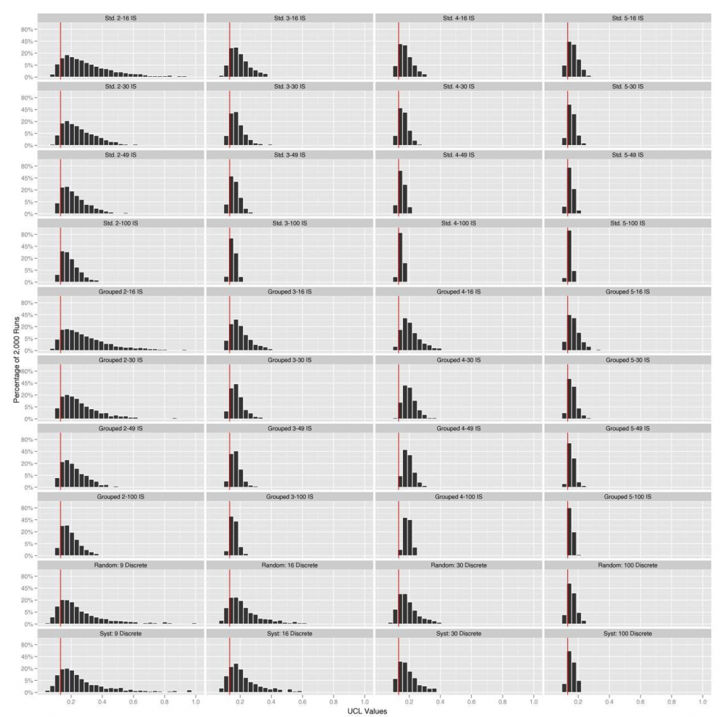
One figure of 40 UCL histograms with consistent axes is shown in each subsection. These figures are meant to show general distributional and coverage patterns of the calculated UCLs over all sampling patterns and may be difficult to use for evaluating any specific one.
The displayed t-distribution UCL calculations are based on a 95% UCL using t-distribution with the df equal to 1 minus the number of measures used to calculate the SD for each scenario. For the ISM sampling patterns, df is the number of ISM replicates gathered from the site minus 1, and for the discrete sampling patterns, df is the number of samples gathered minus 1. It is understood that the t-distribution is not appropriate for cases where the sample size is small and measured values do not follow a normal distribution. This would generally be the case for the discrete sample designs with 9 and 16 samples as applied to the five simulated sites. In many instances, a different UCL method would be needed for all discrete sample designs (16, 30, 49, and 100), and alternative UCL calculations that do not rely on normal theory should be used in those cases. Such UCL calculations can be found in software such as ProUCL (Singh, Maichle, and Armbya 2007) and VSP (Dowson et al. 2007) for use in environmental studies. There are a variety of choices depending on site-specific needs.
For the proposed ISM sampling methods, the t-distribution may not provide adequate coverage, and with the limited number of available data values, it is difficult to use many of the tools in ProUCL for alternative UCL calculations. Thus, a more conservative Chebyshev multiplier is used for attaining an improved coverage percentage; the UCL coverage plots and tables also show the Chebyshev 95% UCL calculations. The SE is multiplied by a prespecified value and added to the mean to identify the UCL. For the t-distribution, this value is a function of the number of values used to estimate the mean and SE. The Chebyshev multiplier is 1/sqrt (1 – 0.95) for a 95% UCL regardless of the sample size used. This generally conservative multiplier of 4.472 will shift the coverage statistics up for all sampling patterns except for the two ISM designs. A t-distribution with 1 df results in a multiplier of 6.313. The most drastic effects of the Chebyshev multiplier are seen with the discrete designs, as their coverage and bias increase the most.
B.4.4.1 Results for RDX (M2-A)
For the RDX (10-m × 10-m DU) simulations, Tables B-5 through B-7 show the summaries from the evaluated simulations. The coverage, bias, number of increments, and number of ISMs are used to create the coverage plot shown in Figure B-11. Figure B-12 shows the panel of 95% t-UCL histograms for all 40 sampling patterns evaluated on the RDX 10-m × 10-m DU.
This site had the strongest small- and large-scale distributional heterogeneity of the two DUs evaluated with a CV of 4.47, with a mean of 71.36 and an SD of 319.1. The coverage results for the standard ISM perform reasonably well for the ISM designs of 100 increments per ISM. The grouped ISM patterns were above the designed criteria of 95% for all but the ISM composed of 16 increments. For this DU, the grouped ISMs are the only patterns that consistently met or exceeded the designed 95% coverage but did have more bias in the mean than the standard ISM or discrete methods.
Table B-7. Discrete summary for RDX DU (M2-A).
Source: J. Hathaway for ACOE, 2012. Used with permission.
| Grid Sampling Type | Number of Increments | Chebyshev 95% UCL Coverage | 95% t-UCL Coverage | Chebyshev RPD above Mean | t RPD above Mean | Chebyshev RPD below Mean | t RPD below Mean |
| Random | 9 | 67.20 | 55.80 | 596.67 | 334.23 | 57.02 | 61.88 |
| Systematic | 9 | 67.65 | 54.90 | 576.75 | 328.07 | 56.18 | 60.07 |
| Random | 16 | 79.25 | 64.50 | 431.13 | 229.60 | 45.61 | 49.98 |
| Systematic | 16 | 81.80 | 65.75 | 425.83 | 229.09 | 47.11 | 48.37 |
| Random | 30 | 84.60 | 67.75 | 292.69 | 145.30 | 34.17 | 40.99 |
| Systematic | 30 | 85.80 | 67.95 | 304.20 | 154.45 | 39.45 | 40.97 |
| Random | 100 | 97.50 | 84.50 | 182.32 | 81.15 | 13.70 | 20.02 |
| Systematic | 100 | 97.95 | 86.80 | 186.52 | 81.02 | 12.22 | 15.26 |
Table B-8. Standard ISM summary for RDX DU (M2-A).
Source: J. Hathaway for ACOE, 2012. Used with permission.
| Number of ISs | Number of Increments | Chebyshev 95% UCL Coverage | 95% t-UCL Coverage | Chebyshev RPD above Mean | t RPD above Mean | Chebyshev RPD below Mean | t RPD below Mean |
| 2 | 16 | 82.95 | 86.35 | 279.99 | 373.67 | 37.86 | 36.14 |
| 3 | 16 | 88.15 | 81.95 | 219.34 | 157.50 | 27.98 | 30.40 |
| 4 | 16 | 92.35 | 82.25 | 199.60 | 122.60 | 24.52 | 26.07 |
| 5 | 16 | 94.00 | 82.45 | 177.73 | 99.96 | 20.89 | 22.80 |
| 2 | 30 | 82.35 | 86.70 | 192.10 | 257.12 | 31.80 | 31.52 |
| 3 | 30 | 90.50 | 83.90 | 150.90 | 105.86 | 23.31 | 24.57 |
| 4 | 30 | 93.65 | 83.95 | 135.61 | 78.51 | 20.59 | 21.45 |
| 5 | 30 | 95.85 | 82.95 | 119.96 | 64.14 | 16.60 | 17.27 |
| 2 | 49 | 87.85 | 90.55 | 147.00 | 200.34 | 25.16 | 23.89 |
| 3 | 49 | 93.20 | 88.30 | 128.19 | 89.26 | 16.46 | 17.75 |
| 4 | 49 | 96.45 | 88.40 | 111.83 | 64.84 | 15.40 | 15.31 |
| 5 | 49 | 96.85 | 88.90 | 101.49 | 53.30 | 14.40 | 15.13 |
| 2 | 100 | 88.10 | 91.10 | 100.46 | 136.07 | 16.05 | 16.26 |
| 3 | 100 | 94.80 | 90.80 | 85.38 | 59.17 | 9.62 | 11.27 |
| 4 | 100 | 97.60 | 92.70 | 76.04 | 43.07 | 7.87 | 10.39 |
| 5 | 100 | 98.30 | 91.70 | 67.41 | 35.27 | 8.17 | 7.79 |
Table B-9. Grouped ISM summary for RDX DU (M2-A).
Source: J. Hathaway for ACOE, 2012. Used with permission.
| Number of ISMs | Number of Increments | Chebyshev 95% UCL Coverage | 95% t-UCL Coverage | Chebyshev RPD above Mean | t RPD above Mean | Chebyshev RPD below Mean | t RPD below Mean |
| 2 | 16 | 90.55 | 93.00 | 408.76 | 560.08 | 41.12 | 42.40 |
| 3 | 16 | 94.90 | 90.75 | 380.21 | 261.11 | 31.43 | 31.17 |
| 4 | 16 | 95.75 | 88.45 | 277.75 | 159.09 | 21.51 | 25.65 |
| 5 | 16 | 97.95 | 92.50 | 297.41 | 152.63 | 17.43 | 23.42 |
| 2 | 30 | 96.05 | 97.85 | 372.63 | 516.93 | 29.51 | 34.85 |
| 3 | 30 | 98.90 | 96.15 | 334.96 | 223.28 | 21.55 | 19.55 |
| 4 | 30 | 99.35 | 95.65 | 239.38 | 128.93 | 13.45 | 18.42 |
| 5 | 30 | 99.80 | 96.20 | 267.77 | 131.54 | 13.41 | 14.40 |
| 2 | 49 | 99.75 | 99.95 | 375.05 | 528.31 | 8.90 | 3.84 |
| 3 | 49 | 100.00 | 100.00 | 342.29 | 222.02 | ||
| 4 | 49 | 99.75 | 98.55 | 240.99 | 127.20 | 7.37 | 17.19 |
| 5 | 49 | 100.00 | 97.50 | 261.90 | 124.83 | 12.04 | |
| 2 | 100 | 100.00 | 100.00 | 374.57 | 528.80 | ||
| 3 | 100 | 100.00 | 100.00 | 336.40 | 217.67 | ||
| 4 | 100 | 100.00 | 100.00 | 238.50 | 125.84 | ||
| 5 | 100 | 100.00 | 100.00 | 266.15 | 126.93 |
Source: J. Hathaway for ACOE, 2012. Used with permission.
Source: J. Hathaway for ACOE, 2012. Used with permission.
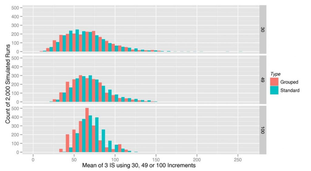
Figure B-13 shows the distribution histograms for the 2,000 estimated means from the grouped and standard sampling patterns. This plot is representative of the other simulated sites and shows a few important highlights. As more increments are included in each ISM, the distribution of means becomes more normally distributed. Both the grouped and standard ISM designs provide unbiased estimates of the mean (71.36) and have virtually identical distributions.
Source: J. Hathaway for ACOE, 2012. Used with permission.
B.4.4.2 Results for HMX (M2-B)
For the HMX (10-m × 10-m DU) simulations, Tables B-8 through B-10 show the summaries from the evaluated simulations. The coverage, bias, number of increments, and number of ISMs are used to create the coverage plot shown in Figure B-14. Figure B-15 shows the panel of t-UCL histograms for all 40 sampling patterns evaluated on the HMX 10-m × 10-m DU.
Table B-10. Discrete summary for HMX DU (M2-B).
Source: J. Hathaway for ACOE, 2012. Used with permission.
| Grid Sampling Type | Number of Increments | Chebyshev 95% UCL Coverage | 95% t-UCL Coverage | Chebyshev RPD above Mean | t RPD above Mean | Chebyshev RPD below Mean | t RPD below Mean |
| Random | 9 | 97.65 | 85.55 | 140.04 | 69.15 | 13.56 | 15.08 |
| Systematic | 9 | 97.40 | 83.70 | 138.07 | 69.42 | 11.88 | 15.48 |
| Random | 16 | 99.05 | 87.00 | 110.39 | 51.50 | 6.36 | 11.33 |
| Systematic | 16 | 98.75 | 86.40 | 108.63 | 50.69 | 5.54 | 13.01 |
| Random | 30 | 99.55 | 87.45 | 83.39 | 37.49 | 4.61 | 8.02 |
| Systematic | 30 | 100.00 | 90.30 | 82.82 | 35.91 | 6.67 | |
| Random | 100 | 100.00 | 92.20 | 48.01 | 19.73 | 4.15 | |
| Systematic | 100 | 100.00 | 92.80 | 47.63 | 19.61 | 4.64 |
Table B-11. Standard ISM summary for HMX DU (M2-B).
Source: J. Hathaway for ACOE, 2012. Used with permission.
| Number of ISMs | Number of Increments | Chebyshev 95% UCL Coverage | 95% t-UCL Coverage | Chebyshev RPD above Mean | t RPD above Mean | Chebyshev RPD below Mean | t RPD below Mean |
| 2 | 16 | 90.70 | 93.60 | 69.45 | 94.49 | 9.84 | 10.13 |
| 3 | 16 | 96.50 | 92.20 | 59.36 | 41.10 | 8.33 | 7.33 |
| 4 | 16 | 97.55 | 90.10 | 52.77 | 30.81 | 5.48 | 6.15 |
| 5 | 16 | 98.85 | 91.75 | 47.53 | 24.89 | 2.97 | 4.66 |
| 2 | 30 | 90.20 | 92.75 | 50.93 | 68.96 | 6.64 | 6.10 |
| 3 | 30 | 96.15 | 92.85 | 40.70 | 27.96 | 5.22 | 5.69 |
| 4 | 30 | 98.20 | 94.00 | 36.95 | 20.86 | 3.59 | 4.59 |
| 5 | 30 | 98.75 | 92.35 | 33.07 | 17.44 | 3.89 | 3.90 |
| 2 | 49 | 90.30 | 92.85 | 39.87 | 54.62 | 6.10 | 6.01 |
| 3 | 49 | 96.40 | 92.35 | 34.71 | 23.86 | 4.60 | 4.47 |
| 4 | 49 | 97.65 | 91.90 | 29.76 | 16.71 | 2.97 | 3.68 |
| 5 | 49 | 98.95 | 92.50 | 26.96 | 13.85 | 2.55 | 3.56 |
| 2 | 100 | 91.40 | 93.30 | 28.15 | 38.71 | 4.67 | 4.69 |
| 3 | 100 | 96.95 | 93.60 | 22.86 | 15.56 | 3.77 | 3.41 |
| 4 | 100 | 98.65 | 94.15 | 20.29 | 11.39 | 1.55 | 2.27 |
| 5 | 100 | 99.10 | 94.05 | 18.50 | 9.47 | 2.10 | 2.24 |
Table B-12. Grouped ISM summary for HMX DU (M2-B).
Source: J. Hathaway for ACOE, 2012. Used with permission.
| Number of ISMs | Number of Increments | Chebyshev 95% UCL Coverage | 95% t-UCL Coverage | Chebyshev RPD above Mean | t RPD above Mean | Chebyshev RPD below Mean | t RPD below Mean |
| 2 | 16 | 90.85 | 92.85 | 70.55 | 96.55 | 9.55 | 8.54 |
| 3 | 16 | 96.95 | 93.05 | 61.46 | 42.15 | 6.42 | 6.05 |
| 4 | 16 | 99.80 | 98.95 | 89.73 | 47.36 | 2.40 | 5.87 |
| 5 | 16 | 99.15 | 93.65 | 52.03 | 26.73 | 5.65 | 5.19 |
| 2 | 30 | 91.20 | 94.00 | 50.99 | 69.54 | 6.84 | 7.05 |
| 3 | 30 | 98.55 | 95.95 | 47.58 | 32.33 | 2.99 | 3.93 |
| 4 | 30 | 100.00 | 99.75 | 87.32 | 46.18 | 3.89 | |
| 5 | 30 | 99.45 | 95.25 | 38.94 | 19.40 | 4.19 | 3.44 |
| 2 | 49 | 92.05 | 95.35 | 38.57 | 52.55 | 5.02 | 5.78 |
| 3 | 49 | 98.70 | 96.75 | 38.65 | 26.05 | 3.67 | 3.43 |
| 4 | 49 | 100.00 | 100.00 | 83.60 | 43.78 | ||
| 5 | 49 | 99.90 | 97.90 | 33.76 | 16.12 | 2.76 | 2.63 |
| 2 | 100 | 93.50 | 95.00 | 29.49 | 40.74 | 5.66 | 5.22 |
| 3 | 100 | 99.20 | 97.15 | 27.85 | 19.02 | 2.88 | 2.07 |
| 4 | 100 | 100.00 | 100.00 | 81.47 | 42.85 | ||
| 5 | 100 | 99.75 | 98.95 | 26.67 | 12.83 | 1.97 | 2.38 |
Source: J. Hathaway for ACOE, 2012. Used with permission.
This DU has some strong distributional heterogeneity, but the distribution of concentration values is not as skewed or heavily right-tailed with a CV of 1.1. The mean is 0.132 with an SD of 0.146. When three or more replicates are used, the coverage results for the grouped ISM patterns were near or above the designed criteria of 95% UCL for all but the ISM composed of 16 increments. The standard ISM performed reasonably well for the 100-increment standard ISM design.
Specific observations from these simulations are noted below and support the consensus points listed in Table B-1:
- The mean concentration estimates for grouped ISM and standard ISM sampling have the same expectation and distribution (see Figure B-13).
- The grouped ISM methods have equivalent or greater coverage than standard ISM when the same number of ISMs and increments are used.
- The RPD of the UCLs for grouped ISM is generally higher than that of standard ISM.
- Grouped ISM, by its definition, provides an improved spatial picture of the concentrations within the site.
- For these maps, the t-UCL may be expected to yield adequate coverage with 100-increment ISM designs.
- As few as 30 increments can be used for DUs with less severe heterogeneity and still maintain coverage with a t-UCL.
- Systematic grid, random grid, or simple random sampling all generally give the same results in terms of coverage, and the use of one or the other can be selected for ease of application (see Figure B-10).
- In general, the Chebyshev method may be necessary to attain adequate coverage depending on the severity of the heterogeneity.
- The improvements in coverage are the more pronounced by increasing the number of increments (for example, 50 to 100) instead of the number of replicates (three to five).
Source: J. Hathaway for ACOE, 2012. Used with permission.
Click Here to download the entire document.


