Systematic Planning, Statistical Analyses, and Costs
The following sections describe the process and considerations involved for DU planning, including statistical analysis and cost estimates.
3.1 Systematic Planning and DU Design
Section 3.1.1 through Section 3.1.5 provides a summary of the key aspects of systematic planning and DU design in relation to the collection of soil and sediment samples. Section 3.1.6 provides three examples that illustrate the application of these key aspects of planning for different types of environmental problems:
- an agricultural field, settling pond, and drainage swale being assessed using screening criteria (Example 1)
- a former agricultural field being converted to residential use (Example 2)
- a former industrial facility that is to be redeveloped, with human health and ecological endpoints (Example 3)
3.1.1 Overview
As with any such sampling event, characterization must generate data in three dimensions so that data needs are met for a range of technical users who participate in the site investigation process. This means collecting data to inform each step of an environmental investigation, including source area identification, evaluation of contaminant fate and transport, and assessment of potential exposure and risks.
ISM-related planning guidance is consistent with USEPA’s DQO guidance (USEPA 2002c), primarily utilizing the first four steps of the DQO process: problem formulation (step 1), identify study goals (step 2), identify information inputs (step 3), and define study boundaries (step 4). Some material associated with step 5 (develop the analytic approach) and step 7 (develop the plan for obtaining data) is also provided in relation to the examples used to demonstrate systematic planning and DU design with ISM. Use of ISM in conjunction with statistical hypothesis tests, which is the focus of DQO steps 5 and 6, is taken up in Example 2 and addressed in detail in Section 3.2.
Note that implementation of ISM does not require that the DQO process be followed. However, to ensure that data obtained during environmental investigations are adequate for their intended purposes, it is strongly recommended that data collection activities be planned and developed through a systematic planning process (SPP) with end users, including the development and consideration of a CSM. Establishing clear objectives at the beginning of the investigation is crucial to efficient and effective site characterization. As described in this section, the outcome of good systematic planning is well-thought-out DUs and SUs (see Section 2.5.1.2), whose locations and dimensions produce information to support all the investigation questions.
USACE’s technical project planning (TPP) process (USACE 1998) provides another example of a systematic planning framework that can readily be used with ISM. More recently, the DQO process has been integrated in the manual for implementation of the Uniform Federal Policy for Quality Assurance Project Plans (USEPA 2005b).A list of guidance documents that can be used with ISM in addition to the DQO, TPP, and uniform federal policy (UFP)-QAPP guidance describing planning processes is provided below:
- “Technical Guidance Manual for the Implementation of the Hawai’i State Contingency Plan” (HDOH 2017b)
- “Improving Environmental Site Remediation Through Performance-Based Environmental Management” (ITRC 2007a)
- “Best Management Practices: Use of Systematic Project Planning Under a Triad Approach for Site Assessment and Cleanup” (USEPA 2010)
- “Triad Implementation Guide” (ITRC 2007b)
3.1.2 DQO step 1: problem formulation (what is the problem, and what decisions need to be made?)
The basic aspects of problem formulation, including establishing the project planning team and developing the CSM, are not unique to investigations employing ISM. When a project team is considering inclusion of ISM as a project tool in the first step of systematic planning, they should consider how ISM might fit into answering related study questions during development of the CSM by calling upon the expertise of a multi-disciplined team (including, for example, chemistry, data analysis, engineering, field sampling, geology, QA, modeling, regulatory, risk assessment, soil science, statistics, and toxicology experts). Important aspects of a CSM for supporting systematic planning are described below, with particular emphasis on applying a CSM for ISM. Additional information on developing and applying CSMs is provided in Section 3 of ITRC’s human health risk assessment guidance (ITRC 2015). USACE Engineer Manual 200-1-12, “Conceptual Site Models,” also provides examples of several different types of CSMs and their use(USACE 2012).
CSMs are essential elements of the SPP for complex environmental problems. They serve to conceptualize the relationships among contaminant sources, environmental fate and transport mechanisms, potential exposure media, and the potential routes of exposure to these media for human and ecological receptors. The structured organization of information to form a CSM creates both a summary of the current understanding of site conditions and anticipates future conditions in a manner that can help the project team identify data gaps in the information needed to make project decisions. These gaps are the basis of study goals (sampling objectives) in the next step of the planning process. In this sense, certain study goals can be thought of as hypotheses related to the CSM, and so achieving sampling objectives serves the purpose of increasing confidence in the CSM.
In addition to a narrative description of these component relationships, a CSM commonly includes pictorial and/or graphical representations of the components of the exposure pathway analysis. Figure 3-1 provides an example of a pictorial CSM depicting a contaminated source area and the pathways through which that contamination travels to reach human health and ecological receptors. Another CSM is rendered in graphical format in Figure 3-2. The pictorial representation of a CSM, such as the example in Figure 3-1, can be particularly useful in risk communication with stakeholders. The graphical depiction, shown in Figure 3-2, is particularly useful for framing study goals and the related inputs and boundaries for supporting site-specific risk assessment. See additional examples in Figures 3-14a and 3-14b.
The CSM may also include summaries of available environmental data, information pertaining to source terms such as listings and quantities of process chemicals, and preliminary transport modeling results.
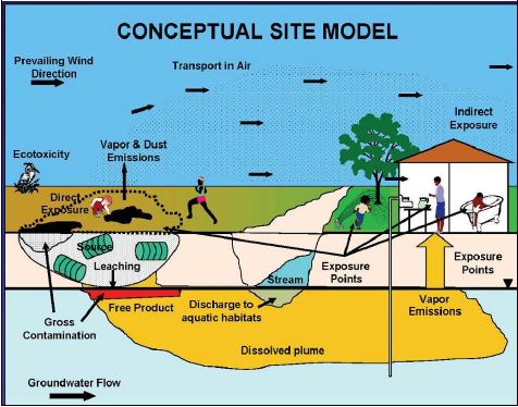
Source: ITRC ISM-1 Team, 2012.
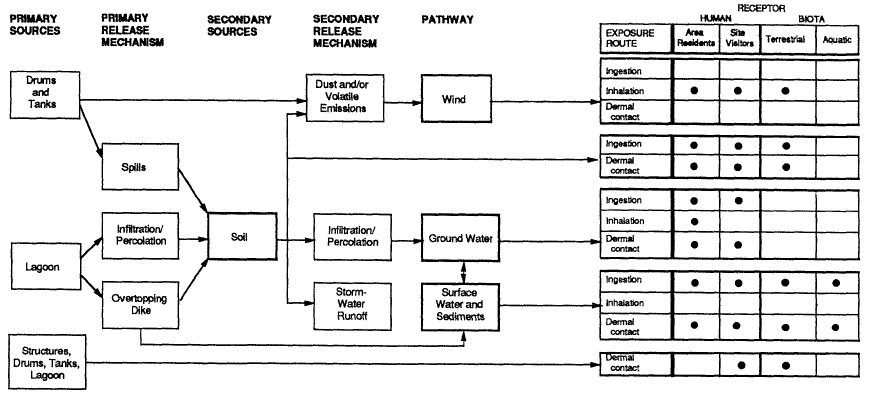
Source: USEPA, 2011.
Decisions about the general sampling approach for a project are crucial in ensuring the data will be adequate to meet project objectives. Project planners may elect to employ ISM or traditional discrete sampling, or even a combination of the two, although these data are not directly comparable and cannot be easily combined (see Section 6.2.5 and Section 6.2.6). The optimum approach depends on the CSM, the sampling objectives, and how the data are to be used. In addition to the technical considerations associated with selecting among different sampling approaches, project planners must also consider relevant regulatory requirements, as well as resource, time, and budget limitations.
Investigation objectives can change as projects progress, which means new information and objectives must continually be reconsidered over the course of the project. Consideration of dynamic or iterative sampling strategies is as essential for ISM as it is for discrete sampling. An example of responding to changing conditions could include establishing additional or alternative DUs to better understand the distribution of contaminant concentrations at a site or to assist in the design and selection of remedial options, based on a review of initial data. Specifically, such a case could involve a relatively large area that was initially thought to be clean and then determined to be heavily contaminated. In this situation, it becomes cost-beneficial to resample subareas in hopes of isolating the contamination and reducing remediation costs. Generally, if DUs are designated in a well-thought-out manner with clear decision statements regarding how the data will be used to answer investigation questions, this will minimize the need for additional unexpected sample collection.
| The CSM is essential for DU design. Determining the size, shape, location, depth, and number of DUs and SUs is a critical component of the planning process and is a function of the CSM, the related study objectives, and ultimately the decision mechanisms that relate to the problem formulation. |
All contaminant concentrations in soil are heterogeneous on some scale (see Section 2), thus the determination of the sampling scale and the related increment density is very important in all sampling situations. If a finer resolution of contaminant distribution is needed to address the objectives of the investigation, then smaller DUs should be considered. Some basic questions that might be considered include, “How do the definitions of DUs and SUs fit to the study goals of the investigation?” and, “How will the resulting data be used in decision-making to solve the environmental problem?” The designation of DUs and SUs should support and clarify the objectives of the investigation. As the investigation proceeds, if study questions are refined or new questions arise, the DUs, SUs, and decision mechanisms should be reevaluated to ensure they will support the decisions that need to be made.
3.1.3 DQO step 2: identifying study goals (what types of additional information do we need?)
As the goals of the study are defined, the project team should consider the suitability of ISM for meeting those goals. ISM is particularly suited to decision problems related to average soil or sediment concentrations. Through the collection of a large number of increments from multiple locations and a relatively large sample mass, ISM provides better coverage and a more robust estimate of average concentrations in a volume of soil than is usually achieved with discrete or traditional composite samples. This is particularly important when contaminant concentrations are believed to be near an action level (AL) or decision threshold, or to resolve disagreements among stakeholders.
Following the identification of the study problem and the development of a CSM, the next step in systematic planning is to identify study goals. This is accomplished by developing principal study questions, based upon the CSM, which, when answered, will allow the user to address the study problem identified in step 1. These questions can vary widely and may be different for different phases of the investigation process within a single project, for example:
- Does soil contamination exist (what is the nature of contamination), and if so, has the extent of soil contamination been delineated?
- Does the average concentration of one or more soil contaminants within the investigation area (IA) present unacceptable risk?
These types of questions can be successfully addressed using ISM. Because ISM is applicable to defined volumes of soil and sediment, it is an ideal tool for assessing risks from soils/sediment, comparing site concentrations to regulatory thresholds or other criteria, bulk material characterization for disposal, or other such problems requiring a high degree of confidence in contaminant concentration in a defined volume of soil/sediment. ISM can also be effective for documenting the presence or absence of significant contamination and establishing whether patterns or trends exist within an IA because it allows the user to efficiently obtain information across a large area.
Once the principal study questions have been developed, the user can develop alternative actions, which are logical responses to each potential outcome of the study question phrased as a decision rule. The process of developing alternative actions allows the project team to develop a consensus-based approach at the onset of the investigation, which minimizes the possibility of disagreements further along in the process. Examples of study questions and decision rules relating to hypothetical site investigations and remedial response are provided in Section 3.1.6.
3.1.4 DQO step 3: identifying information inputs (what are the specific inputs for the missing Information we need to evaluate the study goals?)
Having considered ISM during the formulation of the problem to be solved (step 1) and the decisions to be made (step 2), the project team is in a position to state what information is needed and whether/how the ISM methodology can provide some or all of the data needs pertaining to soil and sediment concentrations. It is in this context that the project team should begin to examine and develop ideas pertaining to the attributes of DUs for ISM sampling.
Project teams may need to identify SUs, or the subdivisions of DUs from which separate ISM samples are collected. The boundaries of an SU indicate the coverage of a single ISM sample –SUs define the scale of the ISM sampling and concentration estimation, whereas DUs define the scale of the decision(s) based on that sampling. These definitions allow for the possibility that ISM samples from several SUs composing a DU can be used collectively to make the decision on that DU. It is also possible to employ SUs to address sampling objectives that do not have a clearly associated DU, such as when sampling to evaluate trends in concentrations with distance or depth from a source. Indeed, information from such sampling may itself be used as an input to redefine a DU’s boundaries. The final criterion of whether an area sampled using ISM is an SU or a DU is whether or not ISM samples from only that area will be used to support a decision.
| SUs define the scale of the ISM sampling and concentration estimation, whereas DUs define the scale of the decision(s) based on that sampling. |
One application of SUs is to collect information about average soil contaminant concentrations in subareas of a DU where soil concentrations are suspected to differ based on the CSM. Similarly, SUs might be used to distinguish subareas of a DU where exposure intensity is expected to differ. In either case, the DU is divided into multiple SUs, each of which is separately sampled with one or more ISM samples. Examples related to the use of SUs in such a manner are provided in Section 3.1.6. A general discussion of the concept of stratification in sampling design is provided in Section 2.5.3.1.
SUs may be advantageously used when sampling a very large area where, due to costs or other limitations, sampling 100% of the footprint of a DU is impossible. For example, a 100-acre DU might be sampled by randomly placing fifteen 1-acre SUs within the DU boundary. In this situation, the SU data are treated in an analogous manner as data from traditional composites or discrete samples to estimate the mean within the DU. As discussed in Section 3.2, ISM data can often be treated as any other data with respect to environmental statistics. An example of how a large DU can be sampled with SUs in this manner is provided in Section 3.1.6.
Caution should be used when applying SUs in ISM study designs. As with other ISM sampling designs, the sizing of DUs should be based on the expected scale of heterogeneity in contaminant concentrations. For example, using a large DU containing non-contiguous SUs may be appropriate to characterize a site where contamination is uniformly distributed based on the CSM, such as aeolian mercury contamination from a power plant or a metals background study. However, such an approach may not be appropriate for a munitions site where range features (target areas, firing lines, and so on) are or were present at the time the contamination was released. For such sites, DUs should be defined for each area representing a unique release profile to aid in site characterization of the nature and extent (N&E). The area and depth of the SU are presumed or already demonstrated through pilot studies to have relatively homogeneous contaminant concentrations that are the results of similar source release mechanisms or dispersion mechanisms.
3.1.5 DQO step 4: define study boundaries (what are the appropriate spatial and temporal boundaries for evaluating the study goals?)
This part of Section 3.1 is the most specific for understanding how to define the number, locations, and dimensions of SUs and DUs to achieve both study goals and support site decisions. The definition of study boundaries for ISM is addressed in the context of informing two interrelated questions that were introduced in Section 3.1.3 as the main objectives of soil and sediment sampling: what is the N&E of contamination, and what is the average contaminant concentration in some defined area?
To address the interdependency of these objectives with ISM, they will be addressed from the premise that understanding patterns of contamination in impacted media as part of an adequate site characterization will assist in designating DU sizes and boundaries. The overarching goal is to determine representative soil contaminant concentrations at a scale that is appropriate for decision-making. For either objective, preliminary data from ISM replicates on the variability of contaminant concentrations can be used to guide delineation of DUs and decisions on the number of increments needed to meet the study goals.
3.1.5.1 Study boundaries related to estimating average soil concentrations in a DU
There are two primary types of DUs that pertain most directly to a study goal of estimating the mean within a defined area: those based on the known locations and dimensions of source areas, called source area DUs or nature and extent DUs (N&E DUs), and those based on the known locations and dimensions of areas within which human or ecological receptors are randomly exposed, called exposure area DUs or simply EUs. In both cases, the primary objective of sampling is to estimate mean contaminant concentrations within a defined volume of soil.
A source area is defined as a discernible volume of soil (or waste or other solid media) containing elevated or potentially elevated concentrations of contaminant in comparison to the surrounding soil such as:
- areas with stained soil, known contamination, or obvious releases
- areas where contaminants were suspected to be stored, handled, or disposed
- areas where sufficient sampling evidence indicates elevated concentrations relative to the surrounding soil over a significant volume of contaminated media
N&E DUs are differentiated from exposure area DUs in that the boundaries of N&E DUs and the scale of sampling are based on a reasonably well-known extent of contamination, while the boundaries of exposure area DUs are determined through the exposure assumptions of the receptors in the risk scenario.
N&E DUs. Source areas are of concern in an environmental investigation because contamination can migrate from source areas to other locations and media (such as leaching to groundwater, volatilizing to soil gas and/or indoor air, overland transport, or running off to surface water), and also because direct exposure to source area contamination may be of concern. The identification and characterization of source areas is an important part of any environmental investigation. N&E DUs can be identified by using various methods, including observation, review of site records, preliminary samples, field analytical samples, wide-area assessments, aerial photographs, interviews, and site surveys. Ideally, source areas are identified based on knowledge of the site before DU designation and subsequent ISM sampling. However, source areas can also be discovered through the interpretation of sampling results.
As discussed in Section 3.1.4, it may be advisable to designate smaller N&E DUs or SUs within larger DUs based on an understanding of potential contaminant distributions. Assessment of a smaller subarea might be motivated by knowledge of site history or topography that could influence fate and transport, leading to an area where concentrations are higher relative to the surrounding soil (that is, a secondary source area). A common example of an N&E DU within a larger DU relates to the investigation of lead soil concentrations in the yards of homes known or suspected to be contaminated with lead-based paint chips. An area around the perimeter of the house might be designated as a separate DU and characterized separately from a larger DU consisting of the entire yard. This is illustrated with an example in Section 3.1.6.2, Example 2B.
Exposure area DUs. Exposure area DUs, or EUs, are a fundamental part of many environmental investigations and are a key tool in risk assessments and risk-based decision-making. An EU in the context of ISM is defined as an area where human or ecological receptors could come into contact with contaminants in soil on a regular basis (refer to exposure area discussion in “Risk Assessment Guidance for Superfund, Vol. I, Human Health Evaluation Manual (Part A)” and “Ecological Risk Assessment Guidance for Superfund; Process for Designing and Conduction Ecological Risk Assessments” (USEPA 1997).
The concentration data collected from an EU can be used to screen risk by using published criteria or to otherwise assess risk to human and ecological receptors. The data are commonly used to develop EPCs, which are generally estimates of the average concentration of a contaminant within the EU. When the remedial decision is to be based on risk assessment results, the EU should represent the area (and depths) where exposure has a high probability of occurring. The size and placement of EUs depend on current use or potential future use of the site, as well as the types of receptors that are expected for each of the land use scenarios. When systematic planning considers soil and sediment data collection to support risk assessment or risk-based decision-making, a primary question is, “Over which area and depth do samples need to be taken to reasonably represent potential exposures of concern?” An EU is commonly a spatially contiguous area within which a human or ecological receptor is generally assumed to be exposed over time in a random manner, and this random pattern of exposure is the basis for using the average to represent the EPC. Practically, we rarely know with a high degree of confidence what the exact size and location of a future exposure area is going to be, although we can make reasonable assumptions or reference default values for certain types of land use. This uncertainty regarding future exposure is why it is important to consider both source areas (based on the known or inferred spatial pattern of contamination) and likely exposure areas in developing DUs.
Lastly, although it is common and practical to discuss EUs based primarily on area, the nature of soil sampling requires that we also consider depth when defining an EU. If, for example, an exposure model states that the activities of humans or burrowing animals might reach a certain depth, then the average soil concentration from the ground surface to that depth is of interest. But here it is especially important to recognize that although, for example, humans could excavate soil to a depth corresponding to a basement, we do not necessarily know they will or what the exact location and volume of the excavation will be. If contamination is surficial, it will generally be inappropriate to assume that future excavation will certainly result in dilution of the contamination through mixing with clean subsurface soil. These ideas concerning EUs are illustrated with examples in Section 3.1.6.
3.1.5.2 Study boundaries related to evaluating the N&E of contamination
ISM can be used to determine the N&E of contamination in soil and sediment at contaminated sites. This section addresses the use of ISM to evaluate the vertical and lateral extent of contamination, and to identify subareas of elevated soil concentrations. The use of ISM in conjunction with field screening tools is also briefly discussed.
Evaluating the vertical extent of contamination with ISM. Subsurface DUs are an important application of ISM sampling because of the frequency with which subsurface contamination is encountered. In some situations, contamination may be situated entirely below the ground surface. Subsurface DUs are often tabular shaped, like thin books, and the number and thickness of these vertical intervals must be carefully considered based on the CSM, site geology/hydrology, potential receptors, existing data, and applicable state regulation and guidance. Objectives for the investigation related to assessing the N&E of contamination in the subsurface might include one or more of the following:
- determining whether leaching of contamination from soil to groundwater may have occurred
- estimating average soil concentrations by depth interval(s)
- estimating the volume of contaminated soil that may need to be removed or properly managed
Ideally, the nature and quality of ISM subsurface samples should be similar to those collected for more easily accessible surface soils, and in a manner that allows every possible increment in the DU an equal likelihood of being collected. Sampling theory also indicates that the entire cross-section of the DU be sampled in each increment making up the ISM sample, but in practice, the combined mass of the increments from a large number of borings would likely result in an impractical sample volume. Therefore, field subsampling plans may be needed to achieve sampling objectives.
Sampling approaches for subsurface soils differ from those applied to surface soils because access to the subsurface is more difficult. It is not uncommon to design an ISM sampling approach for subsurface soils that has less increments than are used in the respective surface investigation, but this does not mean that low-quality data are generated for these subsurface samples. Adequate data can be generated with fewer increments in subsurface sampling when geological heterogeneity and the end use of the data are understood, and this should be addressed during the planning process. Moreover, potential limitations of the data should be clearly discussed, and the implications regarding uncertainty in mean soil concentrations should be taken into account in risk management decisions. Section 4 goes into further detail on sampling techniques for subsurface soils. Example of subsurface sampling designs are provided in Section 3.1.6.
Evaluating the lateral extent of sediment contamination with ISM. When existing ISM data indicate high concentrations of contaminants are locally elevated in soil or sediment, such data may be sufficient to establish the boundaries of a source area. However, in other situations, it may be necessary to refine the study goals and redefine the number and boundaries of DUs based on information from additional sampling.
An example of applying ISM to address data needs pertains to the evaluation of trends in contaminant concentrations as a function of lateral distance. Contiguous ISM SUs along a drainage can provide sound information on contaminant concentration trends and also provide information on average concentrations on the scale of one or more SUs. In some situations, designation and testing of anticipated clean boundary DUs around anticipated areas of heavy contamination can help to minimize the need for remobilization. Examples of an ISM application to evaluate the lateral extent of contamination is provided in Section 3.1.6.
Evaluating the potential presence of subareas of elevated contaminant concentrations with ISM. Historically, discrete soil sample results with concentrations above an AL have often been assumed to represent a significant volume of surrounding soil containing sufficiently high concentrations of contaminant to warrant concern. The concentrations in these assumed volumes have been considered to represent source areas, which are defined in various ways by different regulatory bodies (ITRC 2008). This range of definitions can lead to a wide range of interpretations and has typically led to additional sampling events to further define the N&E as parties struggle to determine what qualifies as an area of elevated concentration versus a source area. It is highly recommended that project teams include their state regulators early in the planning process and that all stakeholders agree upon the basis for defining and distinguishing elevated concentrations from source areas.
One reason why ISM uses so many increments (a minimum of 30) is to have sufficiently dense spatial coverage of the DU. This spatial density improves the chance that the field sample will include significant areas of elevated concentration in the same proportions as present across the DU. An important ISM principle is that DUs should not be designed in a way that results in dilution of significant volumes of highly contaminated soil from smaller areas. The location and size of source areas can often be established or hypothesized based upon site history, including waste disposal units, locations of known or suspected spills or releases, and volumes of soil shown by previous sampling to have significant contaminant concentrations relative to the surrounding soil. In other cases, the presence of subareas of soil with relatively high concentrations is suspected, but the locations are uncertain.
A DQO study goal could be to find significant small areas (horizontal and depth) of elevated contaminant concentration(s) above risk-based concentration(s) or an AL within a DU. The DU could be comprised of several SUs designed to meet the “small area” volume requirement. It is in the systematic planning phase that project teams must define and designate what concentration and what volume, surface area, or mass are significant to their decision-making. To define the size and concentration of a significant small area of elevated contamination, they can use an Excel spreadsheet tool, if the critical condition of a mature CSM is met. For an example and more details on this concept, link to White Paper (Crumbling 2014).
| Statistically based sampling designs can be developed to determine whether localized areas of higher soil concentrations exist, even if the locations of such subareas within a larger site are unknown. |
The spacing of increments (and thus the number of increments needed to fill the DU’s area) can be set to have a desired statistical probability of increments being collected from within an area of defined size for incorporation into the field sample. In this case, if the size of a potential subarea of elevated concentrations is specified, sampling can be conducted to determine whether one or more such areas exist within a DU with an objective degree of confidence and scientific defensibility.
A free software program developed by Pacific Northwest National Laboratory (PNNL) called Visual Sample Plan (VSP) is available to determine the increment spacing for the DU grid so as not to miss sampling from a significant small area of elevated concentrations within the DU (VSP 2019). VSP has varied statistical sample size designs built in to support sample collection using ISM. The designs are grouped into two general categories – estimating the mean and detecting elevated regions. Both designs are built with standard statistical sample size design principles – namely, the stakeholders must specify desired Type I and Type II errors and provide estimates for standard deviations associated with the sampling process as well as regulatory thresholds to which the sample values will be compared. VSP does not implement any of Pitard or Gy’s equations, although it similarly attacks the goal of accurately estimating concentration levels in soil. A validation study of VSP ISM sampling design for elevated regions at a military training range demonstrated reliable estimates of mean concentrations and corroborated spatial areas with statistically elevated concentrations within the DU for 2,4-dinitrotoluene (2,4-DNT) (USEPA, 2015).
VSP’s elevated regions module sampling pattern and design differs from the typical ISM sampling pattern and design described within this document and presented in the examples in both Section 3.1.6 and the case studies in Appendix A. VSP’s elevated regions employ a pattern of rows and columns to design increments for an ISM sample in such a way that they can be combined into ISM samples but still used to spatially locate areas of high contamination. Figure 3-3 depicts a VSP 4 x 4 ISM row-column design with 16 cells. VSP can calculate either the number of incremental samples to achieve a desired power of detecting contamination above a specified level or the probability of detecting an elevated concentration, given a specified number of increment samples.
Source: VSP help file, https://vsp.pnnl.gov/help/.
As with any statistical tool, there are important assumptions and limitations for the user and project team to consider:
- Users must understand the assumptions of the statistical models used in VSP.
- The closer the analyte’s actual data distribution and variability agree with the assumptions of the underlying statistical model, the more accurate VSP’s output will be.
- Even when inputs to statistical calculations are reliable, the numerical outputs of statistical calculations are still imperfect estimates of field concentrations, receptor exposures, and cleanup volumes.
Moreover, there are caveats specific to VSP:
- The user must upload a map of the area (DU) or depict a sampling area (DU) first to enable the ISM Elevated Regions module within the Locate Hot Spots part of a Sampling Goal.
- For very complex shaped sample areas, the site division algorithm does not work well.
- The grids for cells can be square, rectangular, or triangular.
- The user is required to have data on or make a conservative assumption regarding the SD within the small area of elevated concentration and the SD within the remaining IA in the DU. If comparable studies with variance estimates are not available, a pilot study may be needed, which will affect cost. If assumptions on the variance are too conservative, unnecessary costs may be incurred.
- The VSP elevated regions module sampling pattern and design differs from and is more costly than the typical ISM sampling pattern and design, but it provides specific levels of confidence in detecting small areas with significantly elevated concentrations.
- For ISM designs to estimate the mean, VSP does allow the user to input the costs associated with the sample collection and measurement. The costs input are utilized by VSP to propose the most cost-efficient way to aggregate the increments from the DU into the ISM samples with a predicted level of confidence in locating elevated regions in the DU.
During systematic planning, the project team must ensure their study site meets the assumptions and that they have weighed the limitations and caveats for VSP against the study goals. For more details on this concept, see the White Paper (Crumbling 2014). Users are strongly encouraged to fully understand and consult the additional details on VSP designs plus the inherent assumptions and limitations that are available in the VSP help files (https://vsp.pnnl.gov/help/). VSP help for the ISM elevated regions module are under the Sampling Goal menu, Locate Hot Spots, Locate Hot Spots Using MI Samples.
Another approach, but one that lacks the statistical rigor of a defined statistical probability of increments being collected from within an area of defined size, would be to increase the number of increments and thereby the spatial coverage in the DU, to improve the chance that the sample will include significant areas of elevated concentration in the same proportions as present across the DU. A large relative SD (RSD) among replicates can be used as an indication that a small area of elevated concentration in the DU was sampled in one replicate but not in another. This condition might trigger additional investigation with more replicates from the DU, more increments in the DU, or subdividing the DU into multiple smaller SUs. (See Section 3.2.4.2 text and Table 3-2, which classifies heterogeneity of increments in terms of low, medium, and high coefficient of variation [CV] of replicates.)
Effective detection and delineation of areas of elevated concentrations in heterogeneous soil matrices is a challenge. To avoid the pitfalls of “chasing” areas of elevated concentration, ISM practitioners are encouraged to define an area or volume of concern as part of the SPP. Similarly, the planning team is encouraged to define decision rules related to the assessment of the data acquired. An example of such an ISM application is provided in Section 3.1.6.
Use of field screening methods with ISM. Field screening methods can sometimes be used in conjunction with ISM to expedite evaluation of the N&E of soil or sediment contamination. ITRC provides guidance for the selection and use of field site characterization tools to support development of a CSM, plan for the collection of samples for laboratory analysis, and provide input for considering remedial strategies (ITRC 2019). Field portable XRF and gas chromatography are techniques that can be used to gain an understanding of the N&E of contamination and help define the boundaries of SUs or DUs. “EPA Test Method 6200” (USEPA 2007) provides guidance for the use of field portable XRF spectrometry for determining metals concentrations in soil and sediments. Although the guide was written in 2007 and considers the best available technology at that time, its recommendations are valid and still employed in present-day publications and studies. Field portable gas chromatography can be used to evaluate soil and sediment concentrations of organic chemicals, particularly volatile compounds.
3.1.5.3 Laboratory processing of ISM soil and sediment samples
The manner in which soil and sediment samples are processed can affect measured contaminant concentrations in these samples and whether the concentrations are consistent with the assumptions underlying human and ecological exposure models. During the planning process, the project team should consider the physical and chemical characteristics of suspected contamination and the end use of the data to choose the most appropriate sample processing options. There are four issues and related questions that the project team should consider during planning:
- moisture management (Is air-drying of the samples acceptable?)
- particle size selection (Should the samples be sieved or otherwise processed to exclude particles larger than a specified diameter?)
- particle size reduction (Should the samples be ground prior to analysis?)
- sample digestion/extraction (Should the mineral matrix of the sample be dissolved, or should digestion/extraction target the contaminants adsorbed in soil particles or otherwise present in soil?)
The specific analytes that are the focus of the investigation can influence sample processing decisions because there can be a wide range of physical and chemical characteristics within analyte groups. Some characteristics that can influence the selection of sample processing options include boiling point, volatility, air reactivity, and sorption characteristics. The presence of high-concentration nuggets of contamination can also influence sample processing decisions. Section 5.2 provides detailed guidance on selecting sample processing options.
3.1.5.4 Considerations for determining the number of increments and sample mass
As covered in Section 2.5 and Section 2.6, the number of increments collected for an ISM sample and the total mass of the sample are the main factors controlling the representativeness of an ISM soil sample, where representativeness is the measure of how well the sample represents the entire mass of soil within an SU or DU.
Section 2.5 and Section 2.6 should be reviewed to understand the basis for selecting the number of increments for a given sample and the target mass of the ISM sample. Collection and analysis of a large sample mass helps to control what is referred to as CH or FE, which refers to the differences in contaminant concentration related to the physical or chemical characteristics of different soil particles. A large number of increments helps to control distributional heterogeneity, which refers to differences in contaminant concentrations due to the large-scale spatial distribution of contamination within the SU or DU.
The selection of the number of increments and sample mass is dictated by the anticipated degree of small- and large-scale heterogeneity, which might be influenced by the distribution of pockets of contamination across a DU, by contaminant chemical characteristics, by soil type and physical characteristics, and by the contaminant release mechanism.
| It is generally accepted that between 30 and 100 increments is appropriate for many applications, with a larger number of increments being driven by a larger degree of distributional heterogeneity. |
Figure 3-4 presents various factors to consider in deciding on the number of increments to collect from a DU and their influence on heterogeneity. The graphic illustrates the influence of various physical and chemical factors – such as chemical properties, and whether a release is associated with the solid or liquid phase of soil – on potential variability and the related association of each variable to the number of increments to help control heterogeneity.
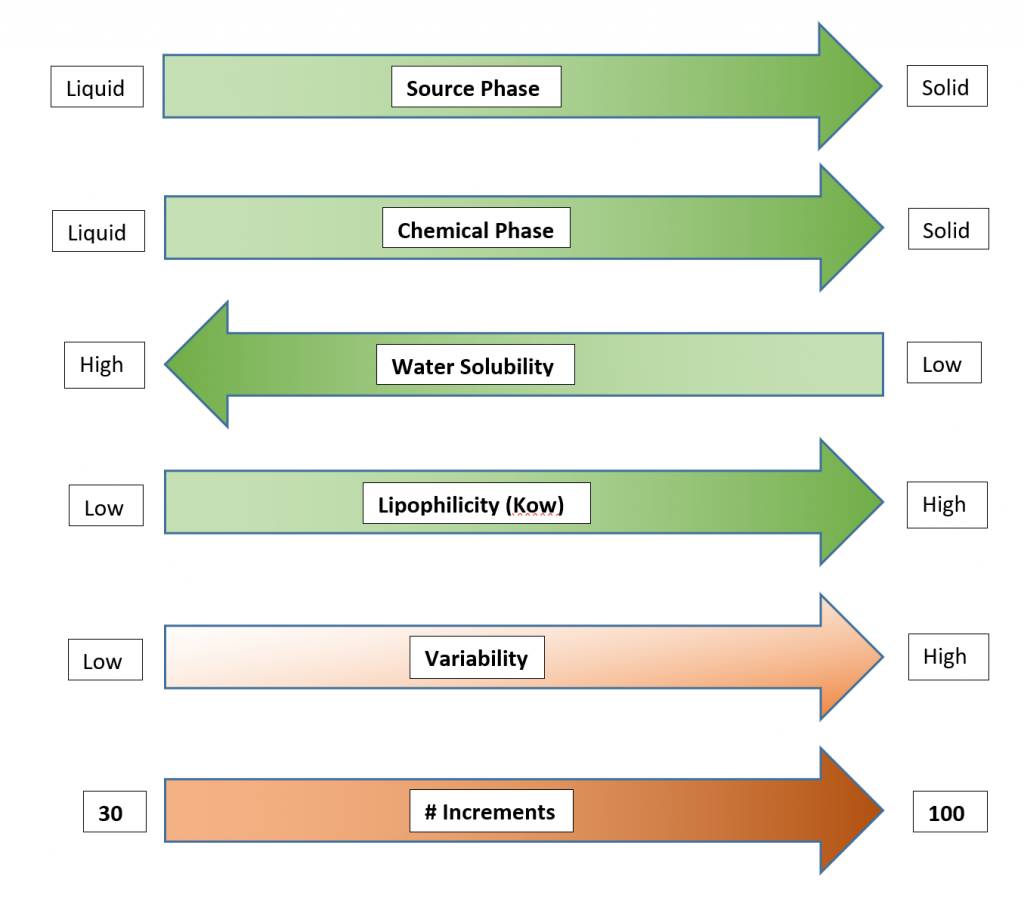
Source: ITRC ISM Update Team, 2020.
Collection of a field sampling mass greater than 1 kg is recommended. Final ISM field samples typically weigh 500 g to 2,500 g, and as discussed in Section 2.5.3.1, many laboratories will limit soil or sediment sample mass to about 2 g to 3 kg. In general, individual soil increments typically weigh 20 g to 60 g. Based on the target final mass of the ISM field sample and the number of increments specified to control distributional heterogeneity, the minimum mass of the individual increments can be calculated (see equation in Section 4.2.3). The mass of any single increment depends on the depth of interest, soil density, moisture content, and the diameter or size of the sample collection tool. In addition to the function of controlling CH, the mass of the final ISM sample must also be sufficient for the planned analyses, any additional QC requirements, and possible repeat analyses due to unanticipated field, laboratory, and/or QC failures. Note that sieving of soil samples at a specified particle size reduces the amount of soil mass available for preparation and analysis, although as discussed in Section 2.6.2.1, such sieving will also tend to reduce CH.
3.1.5.5 Common sampling designs used with ISM
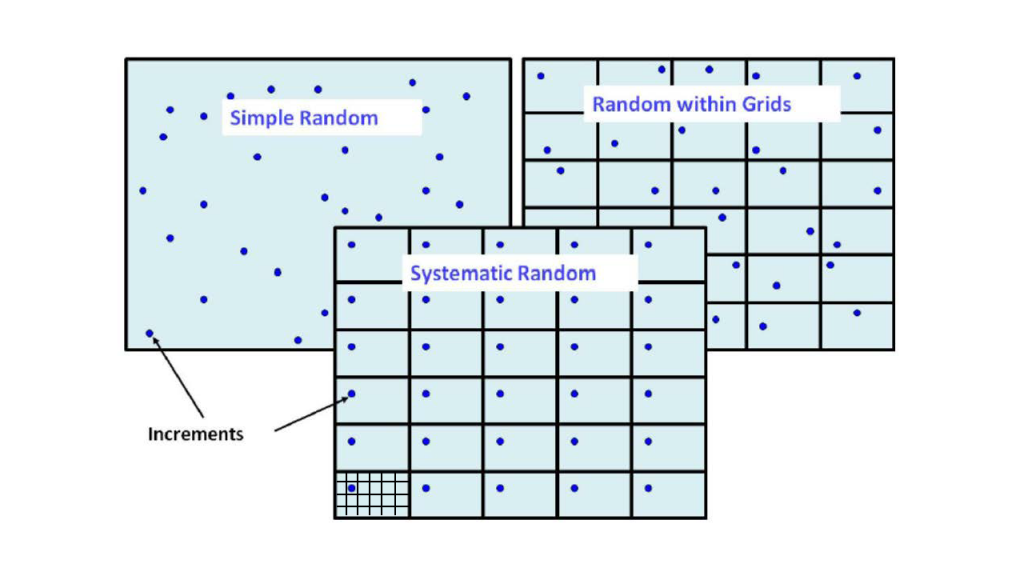
Planning and design for ISM shares many of the characteristics common to other types of environmental soil sampling. Among the common types of statistically based sampling designs are simple random sampling, stratified random sampling, and systematic random sampling. The element of randomness common to these designs allows statistical inferences to be made about the sampled population, as well as a defensible calculation of average contaminant concentrations within a DU. Implementation of these types of sampling designs, along with the basis for selecting among them, is discussed in (USEPA 2002e).
Examples of simple random sampling, stratified random sampling, and systematic random sampling are shown in Figure 3-5. In the case of stratified random sampling, the strata are shown as regular grids, thus the sampling design is labeled “Random within Grids.” For systematic random sampling, rather than selecting a random location for each grid cell within a DU, randomization is performed only once, and the randomly selected location within a cell is then applied to all other cells. This systematic random sampling design is also shown in Appendix A in Case Study 9, which contains a WP with exceptional articulation of the systematic random placement of increments. For further discussion ITRC 2012.
Source: ITRC ISM Update Team, 2020.
Up to this point, this section has provided a summary of the key aspects of systematic planning and DU design in relation to the collection of soil and sediment samples. Section 3.1.6 provides three examples that illustrate these important concepts in different situations.
3.1.6 Examples illustrating planning and design for ISM
The reader will notice that the three examples described here differ in how they were conceptualized and developed. They are presented to illustrate a range of situations and approaches, and to help the reader realize that while thoughtful planning is always necessary, there is no precise formula for how to evaluate a site. Each example illustrates a different application, interpretation, and development of a sampling plan. As discussed in Section 3.1.1, steps 1 through 4 of USEPA’s DQO process have been applied to help structure the discussion of systematic planning and to organize these examples. However, some material associated with later steps of the DQO process (particularly step 7, sampling design) is necessarily integrated in these three examples:
- an agricultural field, settling pond, and drainage swale (Example 1)
- former agricultural field and establishing exposure DUs (Example 2)
- former industrial facility that is to be redeveloped (Example 3)
3.1.6.1 Example 1: agricultural field, settling pond, and drainage swale
Four different ISM topics will be addressed through this example set:
- estimating average concentrations in a defined volume of soil or sediment
- evaluating the vertical profile of contamination in soil or sediment
- evaluating the horizontal extent of contamination along a drainage
- estimating average concentrations in stockpiled material for waste management decisions
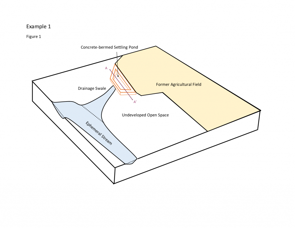
CSM. A bermed enclosure with a cement floor was used for holding irrigation water runoff for a large agricultural field that had not been actively farmed for decades. Water was supplied as flood irrigation to the field, and on occasions when excess irrigation water was applied, the runoff was captured in a 1-acre holding pond situated at a slightly lower elevation than the field. Organochlorine pesticides (OCPs) were historically used on the field, and soil samples from the field indicate that concentrations of several OCPs are above state risk-based soil screening criteria. The farmers note that there is about 6 ft of sediment that has accumulated in the settling pond, and also that the rates of pesticide application had increased over time when the field was being used, such that the more-recent deposits might have the highest concentrations of OCPs. Furthermore, the farmers point out a notch in one of the berms, on the other side of which is a cement apron that leads to a shallow swale. The swale has a gentle gradient and broadens as it leads toward an ephemeral stream that is about a half-mile away. The excess irrigation water reportedly rarely overtopped the berm, but there is little confidence in that observation (see Figure 3-6).
Source: ITRC ISM Update Team, 2020.
Problem formulation. The problem is defined as determining whether sediment concentrations in the settling pond, as well as the swale, could potentially present unacceptable risks to individuals who might currently access the area or to people in the future should the land be repurposed for residential or commercial uses.
Study questions. An initial question (study question 1) is posed as, “Does OCP sediment contamination present unacceptable risk under a residential scenario?”
This question reflects the understanding that residential land use is protective of any other exposure scenario. During the SPP, state soil screening criteria for OCPs are identified as inputs to this question. It is accepted that lateral patterns in OCP sediment concentrations are unlikely within the settling pond, due to the manner in which contamination was deposited, but the CSM’s prediction that the contamination decreases with depth to the cement floor of the settling pond should be confirmed with data. It is further assumed that, because the sediment pond received field runoff directly, OCP concentrations in pond sediments must necessarily be greater than those in the swale.
A second question (study question 2) is therefore posed as, “Are OCP sediment concentrations decreasing with depth in the settling pond?”
Decision rules and sample design for study questions 1 and 2. The first two study questions pertain to OCP sediment concentrations in the settling pond. From these two questions, a decision rule is developed applying the premise that the highest OCP concentrations will be found in the settling pond:
If average OCP sediment concentrations are below residential soil screening criteria in the surface interval, and concentrations are decreasing with depth, then take no further action, else characterize OCP contamination in the swale.
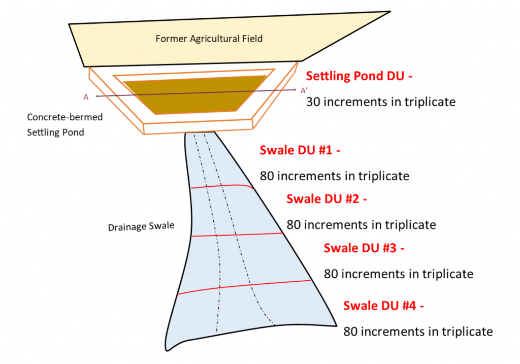
The lateral dimension of the DU area for study questions 1 and 2 is defined as the entire 1-acre surface area of the settling pond within the berms because, as noted in relation to study question 1, systematic patterns in OCP sediment concentrations within a depth stratum are unlikely within the settling pond. For study question 1, a surface sediment interval of 0 to 6 in, where OCP concentrations are expected to be highest based on the CSM, is defined. Because lateral heterogeneity is anticipated to be low, a value of 30 increments is selected from within the recommended range of increments (30 to 100) for the surface soil layer. Three replicates are proposed for the surface interval to support estimation of uncertainty in average OCP sediment concentrations (see Figure 3-7).
Source: ITRC ISM Update Team, 2020.
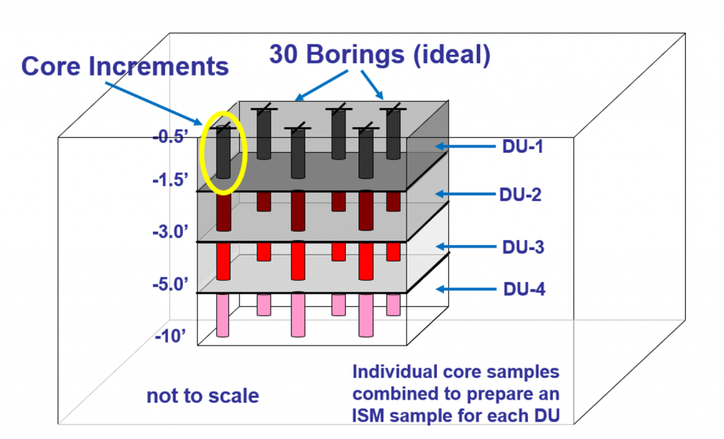
To address study question 2, the remaining depth of sediment (approximately 6 ft) is divided into three depth intervals of approximately 1 to 2 ft each. Although ideally 30 increments and three replicate samples would be collected from the deeper intervals, such as were obtained for the surface interval, the project team decides to phase the depth sampling because of the cost of sampling and the expectation based on the CSM that OCP concentrations at depth are likely to be low and relatively homogenous. Ten corings are proposed to obtain 10 core increments from each of three subsurface intervals corresponding to the approximate 6-ft sediment depth in the settling pond (0.5-1.5 ft, 1.5-3 ft, and 3-5 ft), with no replicates. Figure 3-8 depicts DUs pertaining to subsurface sampling, where DU-1, DU-2, and DU-3 are applicable to Example 1. A 1-kg sample is identified for collection as a plug subsamples from each of the three depth increment (see Section 4.5.1), resulting in a 10-kg sample mass for each subsurface interval. Because laboratories typically limit sample mass to a few kg, field subsampling (per discussion in Section 5.3.5) is proposed for the 10-kg samples to prepare a final 2-kg sample for shipping to the analytical laboratory. A second decision rule is developed specific to study question 2:
If OCP sediment concentrations in a depth interval are clearly below residential soil screening criteria, then take no further action, else consider either additional sampling to refine the estimate of average OCP concentrations (if concentrations are close to criteria) or remedial action (if concentrations are far above criteria).
When the settling pond analytical data for OCPs are received and evaluated, two key findings emerge. First, it is clear that OCP concentrations in all depth intervals exceed both residential and industrial state soil screening criteria. Also, there is relatively high variability among the three replicate samples of the surface sample interval, meaning the assumption of relatively homogeneous contamination seems to be incorrect. Based on the magnitude of the screening level exceedances, it was determined that proceeding with this relatively large degree of data variability was unlikely to result in decision errors, and that the data were sufficient to proceed to consideration of remedial action in the settling pond without further sampling (see study question 4 below).
Source: ITRC ISM-1 Team, 2012.
Decision rule and sample design for study question 3. Consistent with the decision rule for study questions 1 and 2, a design is developed to evaluate OCP contamination in the swale. The swale is divided longitudinally into 500-ft intervals between the settling pond and the ephemeral stream. As the swale broadens with distance from the pond, the areas of these swale segments also increase with distance: 5,500 ft2, 8,000 ft2, 15,000 ft2, 19,000 ft2, and so on. There is no visual indication of channeling or deposition within the swale. The range of surface areas in the first four swale segments, from about one-eighth to one-half-acre, are sized to fall within the range of areas applicable to both human and ecological exposure scenarios related to state soil screening criteria. Because there is no visual evidence of preferential areas of sediment deposition in the swale, and because the areas of the swale segments are within the range of potential exposure areas, there is minimal concern that there could be subareas of higher concentrations or hot spots within a swale segment. Therefore, contingencies for defining smaller DUs based on data evaluation are not proposed. The residential soil screening criteria applied for the decision rule for study questions 1 and 2 are also applied to the swale segments, since they are determined to be protective of potential ecological impacts.
A third study question (study question 3) is developed: “Do average OCP sediment concentrations in the swale present unacceptable human or ecological risk, and if so, has the lateral extent of contamination relative to such concentrations been established?” From this question, the following decision rule is developed:
If OCP sediment concentrations are decreasing with distance from the settling pond, and average OCP concentrations are below residential soil screening criteria, then take no further action in the swale, else consider additional sampling (to determine extent) and/or site-specific risk assessment or remedial action.
Each of the first four swale segments are defined as DUs. A sediment depth interval of 0 to 12 in is defined for sampling, based on a field survey that showed roughly this thickness of fine-grained material (similar to agricultural field soil) is present within the swale. Because heterogeneity of OCP concentrations in swale sediments is unknown, and given higher than anticipated heterogeneity in settling pond sediments, a value of 80 increments is selected from within the recommended range of increments (30 to 100). Three replicates are proposed for all four segments.
When the swale segment analytical data for OCPs are received and evaluated, OCPs are detected sporadically and only in the first two segments. The average concentrations of OCPs in these segments are below both residential and ecological screening criteria, so consistent with the decision rule for study question 3, no further action is proposed for the swale.
Decision rule and sample design for study question 4. As discussed, average OCP concentrations in all depth intervals of the settling pond exceed screening criteria by a relatively large margin, and evaluation of the three replicate data for the surface interval indicates that there is a high degree of variability in OCP sediment concentrations. Rather than continue in situ sampling, informal cost-benefit consideration suggests that it is advisable to excavate settling pond sediments and dispose of them in an appropriate facility. The OCP concentrations are near levels that differentiate between two disposal facility options with very different disposal costs. An excavation and stockpiling plan is developed to remove sediments by depth and stage them in a long and narrow stockpile that is arranged on the long axis from shallower to deeper sediments, since the analytical data indicate an inverse relationship between OCP concentration and depth.
A fourth study question (study question 4) is developed: “Are average OCP concentrations in segments of the stockpile above the acceptance criteria of the lower-priced landfill?” From this question, the following decision rule is developed:
If average OCP sediment concentrations in a stockpile segment are above the acceptance criteria of the lower-priced landfill, then send the material to the higher-priced landfill, else ship to the lower-priced one.
The volume of an individual stockpile segment, defined as a stockpile DU, is determined by transportation costs and minimal disposal quantity rules for the hazardous waste landfill. The stockpile is laid out with a depth of 2 ft to allow for cost-effective hand coring. Because heterogeneity is known to be high, and sampling costs are low, a value of 100 increments per segment is selected from within the recommended range of increments (30 to 100). Three replicates are proposed for all segments to support an estimate of a 95% UCL on mean OCP concentrations.
3.1.6.2 Example 2: former agricultural field and establishing exposure DUs
Example 2 focuses on developing and delineating EUs for human health risk-based study questions and will guide you through the development of ISM sampling plans with successively more complex site CSMs. Throughout Example 2, the risk-based study questions focus on current and potential future residential land use with no ecological receptors. The DU size is ¼ acre, the assumed size of a future residential lot. Residential lot sizes vary, thus planning with a regulatory authority and their risk assessor is essential.
Example 2A covers four concepts:
- establishing replicate heterogeneity limits in the DQOs as an MQO in Specific Study Goal data needs
- assessing the assumption of homogeneous contaminant distribution (low heterogeneity) by defining as RSD of 20% in a Decision Rule.
- extrapolating to unsampled DUs within a large study area
- designing background DUs
Example 2B covers three additional concepts:
- Designing source area N&E DUs within EUs
- Designing SUs within DUs (for example, a children’s play area within an adult residential DU)
- Designing for weighted averaging of 95% UCL
The problem formation (DQO step 1) is similar for both Examples 2A and 2B: determine the average concentrations of COPCs in surface soil to assess if potential risks are unacceptable to current and/or future residents. (Note that Example 1 provides guidance on subsurface sampling. Care should be taken to plan for the number of subsurface increments needed to obtain reliable concentration estimates with minimal uncertainty, like surface soil ISM sampling, for use in estimating potential risks.)
Example 2A. The CSM for Example 2A (Figure 3-9a) is a 30-acre agricultural use area that has been farmed since the early 1900s. Legal broadcast application of OCPs and arsenical pesticides, including lead arsenate, is the only suspected potential source of soil contamination and is limited to surface soil contamination with no migration of COPCs to the subsurface. The topography is flat, except for furrows between rows of plants. No localized areas of potentially heavy contamination were identified in a thorough Phase I Environmental Site Assessment (ESA). Moreover, county records indicate that, in recent years, there has been no use of triazine herbicides, carbamates, or organophosphate pesticides. There are no known or suspected pesticide mixing areas, and no existing structures or historical aerial photographs show any evidence of structures dating back to the 1920s. The site is surrounded by agricultural fields, except an area to the west that has never been farmed or had any other known uses based on historical photographs and county records. The site is scheduled to undergo residential development.
Problem Formulation – Identify decisions needed and develop CSM. The goal of the ISM sampling event is to determine the average concentrations expressed as the 95% UCL of arsenic, lead, and OCPs in surface soil to assess potential future residential risks and ascertain if cumulative risks or hazards exceed the regulatory acceptable points of departure of 1 x 10⁻⁶ and 1.0, respectively (see Section 1, where 95% UCL is defined, and Section 3.2, which has a discussion on 95% UCL).
For risk-related problems, problem formation will almost always entail the following sequence of steps to generate the preliminary CSM and potentially complete exposure pathways:
- identify potential primary source areas/release mechanisms
- identify potential secondary source areas/release mechanisms
- identify media that could be impacted by such a release/migration (exposure media)
- identify receptors, both current and future, that could come into contact with these contaminated media and the exposure routes (ingestion, inhalation, or dermal)
First, generate the preliminary CSM and potentially complete exposure pathways to establish EUs.
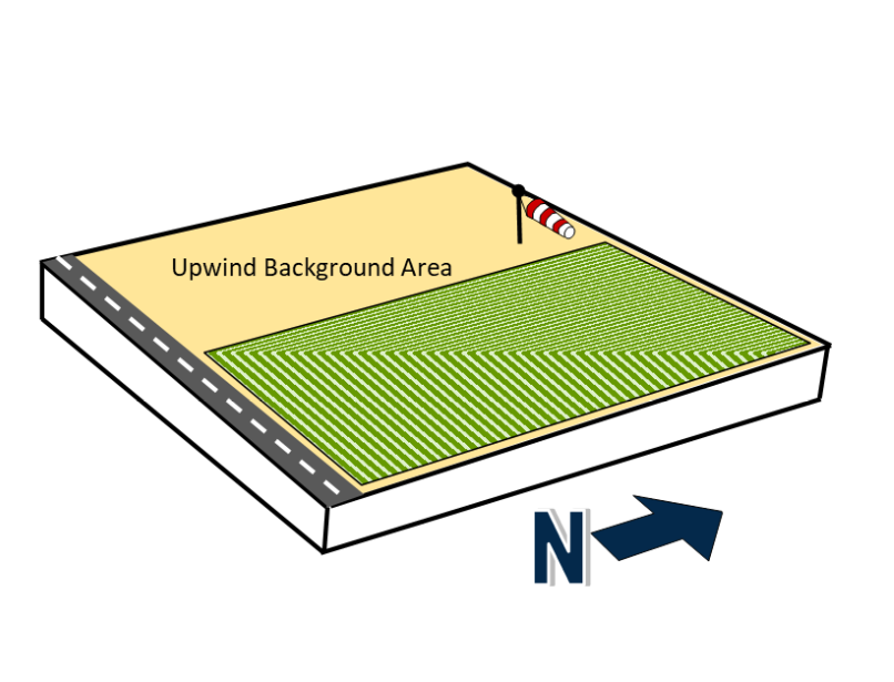
- Primary source areas/release mechanisms. The only potential source for Example 2A is the agricultural field, with the release mechanism being the legal broadcast application of OCPs and arsenical pesticides, including lead arsenate. There have been no known releases to the adjacent background area that is upwind from the agricultural field.
Source: ITRC ISM Update Team, 2020.
- Secondary source areas/release mechanisms. The broadcast application of pesticides leads to contaminated soils as a secondary source. Secondary releases of COPCs from surface soil can occur from transport of these non-volatile COPCs in surface soil via wind dispersion and plowing of the agricultural field.
- Exposure media. The exposure media are limited to surface soil (defined as the top 6 in).
- Receptors and routes of exposure. Future residential receptors may be exposed to COPCs in surface soil via incidental ingestion, inhalation of particulates, and dermal contact.
Identify Study Questions – Identify objectives and COPCs. To determine what environmental data are needed to achieve the goals of the ISM investigation, the project team develops the study questions that will guide the sampling and analysis plan in conjunction with the CSM. Example 2A has two study questions; the resulting decision rules are used to develop consensus on ISM results-based actions to help define the data quality needs:
- Study question 1 – Are the average metals concentrations expressed as the 95% UCL in the agricultural field within ambient background concentrations?
- Decision rule 1 – If the 95% UCL soil metals concentrations are within ambient background concentrations, then do not include metals in the risk assessment, if not, include metals as COPCs in the quantitative risk assessment.
- Study question 2 – For each EU in the agricultural field, are the average concentrations expressed as the 95% UCL for each OCP and each metal below risk-based levels of concern?
- Decision rule 2.1 – If OCPs are not detected in surface soil and all metals are identified as within ambient background concentrations, then no further action, if not, proceed to decision rule 2.2.
- Decision rule 2.2 – If replicate RSDs of risk-driving COPCs exceed measurement quality objectives (MQOs), then further investigation, if not, calculate cumulative risks and hazards and proceed to decision rule 2.3.
- Decision rule 2.3 – If cumulative risks and hazards in any EU are above the regulatory acceptable points of departure for risk (1 x 10⁻⁶) and hazard (1.0), then for all EUs further action or investigation, if not, no further action.
Identify Information Inputs – Specify study goal data needs. Two information inputs are identified for Example 2A.
- Surface soil sampling and analysis are needed for OCPs and metals with detection limits below risk-based screening levels from ¼-acre EUs.
- Define MQOs, particularly the acceptable range of replicate RSDs. For example set 2A, an RSD of less than 20% is established as the MQO.
Define Spatial and Temporal Study Boundaries – Define DUs. The study area’s lateral boundary is the 30 acres of agricultural land that is proposed for residential development. The vertical boundary is defined as surface soil based on the release mechanism of broadcast pesticide application and the relatively low mobility of OCP pesticides in soil. Because the study questions are risk-based, the DUs are defined by the anticipated exposure areas, described above as ¼-acre EUs.
| Extrapolating to unsampled DUs within a large study area can be achieved in a scientifically defensible manner with ISM. |
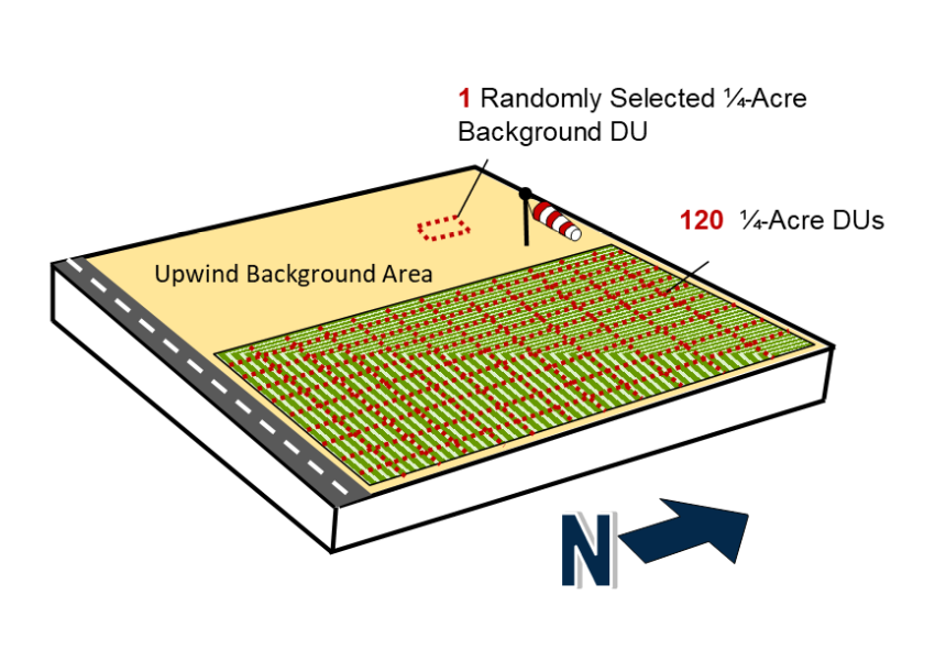
Extrapolating to unsampled DUs within a large study area can be achieved in a scientifically defensible manner with ISM. Section 3.1.3 and Section 3.1.4 touch on the concept of sampling a subset of SUs within a large DU. This concept is applied in this example to extrapolating conclusions from a subset of sampled DUs to a larger group of CSM-equivalent DUs, as described in more detail in Section 3.2.8.2. The utility of a pilot study for large areas to assess variability and obtain preliminary COPC concentration ranges is typically very beneficial. In this example, low variance among replicates is anticipated based on the CSM of broadcast pesticide applications, and the 30-acre study area is divided into 120 contiguous equally-sized DUs of a ¼ acre (Figure 3-9b) based on the residential lot size in the area. A subset of DUs can be randomly selected (such as with a random number generator) for sampling. Alternatively, a modified random selection process can be used to ensure that all regions of the 30-acre area are sampled in a proportional manner to reduce the uncertainty from extrapolation if the subset of DUs identified for sampling are grouped too closely together. For modified random selection, the 120 DUs would be allotted into spatial groups and equal numbers of DUs for sampling selected from each group.
Source: ITRC ISM Update Team, 2020.
Planning for the number of DUs to sample as the subset of the 120 DUs is a decision that involves all stakeholders and most critically must be sufficient to support the ultimate decisions made based on the extrapolated contaminant average concentration data. Example 2A decisions will be risk-based decisions, and considerations for addressing uncertainty in the risk estimates and risk-based decision errors should err on the side of protecting public health. Generally, practitioners would rather make the mistake of remediating a site that is already clean than make the mistake of not remediating a site that is contaminated.
As presented in Section 3.2.8.2, based on the statistical equations for upper tolerance limits (UTLs) using nonparametric methods, when there are a large number of DUs (more than 100), a subset of at least 59 DUs must be sampled to conclude that at least 95% of the site area is in compliance with 95% confidence (0.05 = α). From a practical standpoint, confidence in making correct decisions about a large-area site will increase as the proportion of the site area included in ISM sampling increases. Section 3.2.8.2 describes the statistical basis that supports sampling designs that can achieve specified decision error rates, given properties of the data and key assumptions. Based on these numerical simulation studies and statistics commonly applied in environmental investigations, there are conditions when compliance can be achieved by sampling a small portion of the study area (for example, 10% to 30%). The decision regarding the number of small-area DUs to sample should be based on spatial coverage (representativeness) of the site area, the likely degree of variability in soil concentrations across the site area, and the likely proximity of soil concentrations to ALs.
For Example 2A, the project team agrees to determine which DUs to sample using modified random selection and to sample 20 DUs (17% of the total site area, or 5 acres from the 30 acres). This decision to sample 20 DUs by the project team is informed by similar nearby study areas with thorough investigations that had a low CV (<1) and COPC concentrations between 10- and 100-fold lower than risk-based screening levels for all DUs. Therefore, sampling 17% of the site area, or 20 DUs, should be sufficient to avoid a high rate of false compliance decisions while achieving cost savings relative to sampling 59 DUs. Furthermore, the project team agrees that if the CSM assumptions are proven incorrect with either (1) high RSD between replicates or (2) high variability among DUs, then further investigation will ensue with sampling of additional DUs and/or sampling with more increments per DU, rather than extrapolation of the results to the remaining 100 DUs. The anticipated COPC concentrations (that is, 95% UCL to AL ratio of 0.01 to 0.1) plus these two caveats help reduce the uncertainty in drawing conclusions from sampled DUs to other DUs at the site.
Planning by the project team for the number of increments to sample should consider multiple factors. ISM applies soil science and Gy’s theory to reduce soil sampling heterogeneity and thereby decrease variability in soil contaminant concentrations among increments and replicates. ISM variability can be reduced by increasing the number of increments collected for an ISM replicate, as described in Section 2. Some of the factors that contribute to heterogeneity in soil contaminant concentrations are taken into consideration when establishing DU boundaries, such as the location of the primary source and secondary or tertiary sources and the soil depths of interest to answering the project team’s study questions. Some key factors to consider in deciding on the number of increments in systematic planning are the primary sources and the physical phases of the primary sources (solid or liquid), as well as physical (solid or liquid phase) and chemical properties (water solubility and lipophilicity) that affect COPC fate and transport. The effect of these variables on the heterogeneity in soil contaminant concentrations and the number of increments that should be collected within a DU are illustrated in Figure 3-4. A minimum of 30 increments should be used for each ISM sample or replicate – up to 100 increments may be necessary for some sources/COPCs. The minimum of 30 increments is based on statistical simulations and over a decade of practitioner experience (see Section 2). For certain source types and chemical classes (such as munition residues, metals at small-arms firing ranges, paint chips, ash with dioxins/furans, polynuclear aromatic hydrocarbons [PAHs], and PCBs in transformer oil), more than 30 increments may be necessary due to the highly heterogeneous way these contaminants can be distributed in soil. Case Study 3 in Appendix A demonstrated that 50 increments were insufficient for benzo(a)pyrene (BaP) from a landfill source. Case Study 2 (Clausen et al. 2018a) in Appendix A investigated various numbers of increments (5, 10, 20, 30, 50 100, and 200) to determine how the number of increments affect data quality and concluded ISM samples with 100 increments were appropriate. A field investigation on a diverse set of sources and COPCs from three different sites was undertaken by Brewer et al (Brewer, Peard, and Heskett 2016), which concluded that the magnitude of variability depends in part on the contaminant type and the nature of the release. The sites were (A) a former manufacturer of arsenic-treated ceiling and wall boards, (B) a former municipal incinerator, and (C) a former radio broadcasting station with releases of arsenic, lead, and PCBs in oil, respectively. Variability was well managed for arsenic (site A) and lead (site B), where the use of 54 increments each resulted in RSDs of 6.5% and 20%, respectively. The concentration of PCBs from transformer oil (site C) was so heterogeneous that even in a very small DU, 60 increments were not enough to address the distributional heterogeneity with an RSD of 138%.
For Example 2A, the project team decides to collect three replicates of 50 increments within each of the 20 DUs. Although 30 increments may be sufficient for broadcast application of water-based pesticides that contain arsenic or lead, the use of 50 increments per ISM replicate is decided by the project team to increase the ISM replicate mass because OCPs are hydrophobic (having low water solubility) and have been demonstrated to have relatively large small-scale variability (leading to a higher degree of variability among the increments) at a nearby agricultural field. Table 3-1 presents the variables considered by the project team to determine the number of increments per DU in the agricultural field for Example 2A.
Table 3-1. Variables considered in determining the number of increments per DU for Example 2.
Source: ITRC ISM Update Team, 2020.
| Area | Source(s) | COPCs | # Increments | Rationale |
| Agricultural Field | Pesticides application (lead arsenate) | Arsenic | 30 | Water-based pesticides |
| Pesticides application (OCPs) | OCPs | 50 | Hydrophobic COPCs | |
| Pesticide Mixing | Spills or ground surface disposal | Full suite of pesticides and petroleum fractions | 70 | Brewer et al., 2016 (PCBs n > 60) n = 70 to 100 |
| Residential Area: Current (Example 2B-1) | Paint chips | Metals (lead) | 80 | Hawaii DOH, 2016 (n > 75) |
| Termiticides | OCPs | 80 | Brewer et al., 2016 (PCBs n > 60) n = 70 to 100 |
|
| Pesticide drift (lead arsenate and OCPs) | Arsenic and OCPs | 80 | Efficiency of one sampling strategy Unknown heterogeneity (n = 50, Hawaii DOH, 2016) | |
| Residential Area: Future (Example 2B-2) | Paint chips | Metals (lead) | 80 | Hawaii DOH, 2016 (n > 75) |
| Termiticides | OCPs | 80 | Brewer et al., 2016 (PCBs n > 60) n = 70 to 100 |
|
| Pesticide drift (lead arsenate and OCPs) | Arsenic and OCPs | 50 | Efficiency DUs 1 to 4 for one sampling strategy Unknown heterogeneity (n = 50, Hawaii DOH, 2016) |
|
| Dump Area Debris | Tires, 55-gallon drums of unknown contents, ash, oil-stained soil, debris | Metals, OCPs, full suite of pesticides, SVOCs, PAHs, dioxins/furans, petroleum fractions | 80 | Brewer et al., 2016 (PCBs n > 60, ash lead n = 50 to 60) Sources and COPCs suggest high heterogeneity n = 70 to 100 |
The three replicate locations are established by using systematic random placement as per Section 3.1.5.4 (Figure 3-5), with each DU divided into 50 equally-sized grids. For systematic random selection, after the initial three replicate location is randomly selected, this placement is applied to the remaining 49 grid cells for that DU. If the increments unevenly represent the furrows or crests of the rows, then discuss with the regulatory team the use of a modified systematic random selection process for placement of increments. Similarly, contingencies may be needed if increment locations are inaccessible due to the physical presence of crop vegetation (see Section 4).
Defining background DUs is a concept important for both risk assessment and risk management. Background soil concentrations for native metals and ubiquitous anthropogenic chemicals such as dioxins and PAHs are often used in risk assessment (see Section 8.4) to establish cleanup goals or verify remedial actions. Background DUs need to be of comparable area and depth (volume) as the site DUs and from a geologically similar area with no known or suspected sources of contamination. ISM background samples need to be of equal sample support – that is, both the field increment volume and number of increments and laboratory subsampling protocols need to match those of the site ISM samples. Ideally, ISM background samples should be comparable to site data and share the attributes of:
- same DU size (volume)
- same sample range of depths
- same soil type (such as sand or loam)
- same volume of soil per increment
- same number of increments and replicates in the DU
- same increment density (such as 30 increments per ½ acre; see Figure 3-10)
- same field methods
- same analytical methods
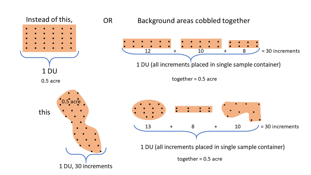
In situations where nearby background regions are difficult to find, areas equal to the site’s DUs from irregularly shaped regions or a combination of discontinuous regions are alternatives (see Figure 3-10 with an example of a background 0.5-acre DU). If different soil types exist within the site, or if soils are derived from different parent material, then multiple ISM background datasets may be needed with one for each soil type.
Source: ITRC ISM Update Team, 2020.
The upwind background area in Figure 3-9a is ideal to avoid any potential cross-contamination from wind deposition during pesticide applications, plowing activities, or windy events. The background sampling must consist of the same number of replicates per DU as the study area, which in Example 2A is three replicates. For Example 2A, one ¼-acre DU is selected from the background area to collect the three replicates of 50 increments each (Figure 3-9b). Similar to the agricultural area DUs described above, the background three replicate locations are established using systematic random placement with the background DU divided into 50 equally-sized areas.
Example 2B. The CSM for Example 2B is a 32-acre parcel proposed for residential redevelopment with a 30-acre agricultural use area, per Example 2A with additional site features and potential source areas (Figure 3-11a). All sources are releases at ground surface. In addition to the legal broadcast application of OCPs and arsenical pesticides, including lead arsenate, the Phase I ESA identified other potential source areas. The parcel had one or more potential pesticide mixing areas, with one currently visible adjacent to an agricultural well that has been present since the 1930s. A rural residence (house) on an acre of the parcel was built in the 1940s, and there is a children’s play area of approximately 0.02 acres (approximately 870 ft2) that includes a swing set in a bare dirt area. The surrounding agricultural land on the parcel is leased and not farmed by the current occupants. A low-lying area exists in the northeast of the parcel that contains debris from miscellaneous illegal dumping of tires, multiple 55-gallon drums of unknown contents, ash, and oil-stained surface soil. The dump area is approximately 1 acre. There have been no investigations of similar nearby study areas to inform the team on expected COPC concentrations.
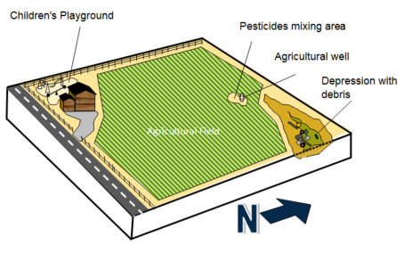
Source: ITRC ISM Update Team, 2020.
Agricultural mixing areas are potential sources of localized heavy contamination of OCPs, arsenic, and lead. Conditions of potential contaminant distribution in pesticide mixing are much more uncertain than in other areas of the agricultural field. In addition to direct exposure hazards, contamination could also pose leaching hazards and subsequent contamination of underlying groundwater resources. Triazine herbicides, arsenic, and other chemicals can pose additional leaching threats to underlying groundwater. While ISM is useful for determining average concentrations of COPCs over a volume of soil and modeling for leaching, it is beyond the scope of this example. Pesticide mixing areas should include the full range of pesticides as COPCs and petroleum fractions.
Potential sources of chemical contamination surrounding the residential structure are lead-based paint and organochlorine termiticide applications around the base of the foundation. The debris/dump area COPCs are SVOCs, including PAHs, metals, dioxins/furans, and petroleum fractions.
Preliminary data have shown site soil arsenic and lead concentrations are above ambient background soil concentrations. Thus, comparison to background is unwarranted as both arsenic and lead will be carried through the risk assessment as COPCs. Although PAHs are ubiquitous in the environment, the ambient concentrations of PAHs are expected to be very low and have no effect on the risk in Example 2B due to the rural location of the site and lack of generalized local source dispersion. Applicable background data for site-related organic chemicals are unavailable, and the project team has decided to review initial risk results to support whether future background studies for other analytes are consequential.
The project team agrees to a phased approach, with the Phase I investigation limited to surface soils based on the sources of release all being to ground surface. The team agrees that if cumulative risks and hazards in any EU are above the regulatory acceptable points of departure for risk (1 x 10⁻⁶) and hazard (1.0), then a Phase II investigation will ensue. The remainder of Example 2B focuses on unique aspects not included in Example 2A and is largely directed to defining the EUs.
Problem Formulation – Identify decisions needed and develop CSM. The goal of the ISM sampling event is the same as in Example 2A, to determine the average concentrations of COPCs expressed as the 95% UCL in surface soil for use to assess potential current and/or future residential risks and ascertain if cumulative risks or hazards exceed the regulatory acceptable points of departure of 1 x 10⁻⁶ and 1, respectively. All sources are releases at ground surface, and the decision rules specify additional investigation if surface soil risks are above regulatory thresholds. COPCs in Example 2B include OCPs, the full suite of pesticides, arsenic, lead, SVOCs, PAHs, dioxins/furans, and petroleum fractions.
The Example 2B preliminary CSM includes the aspects from Example 2A’s agricultural field. The exposure media as well as the receptors and routes of exposure are the same as Example 2A.
- Primary source areas/release mechanisms. There are four primary source areas/release mechanisms:
- Agricultural field. This potential primary source release mechanism was the legal broadcast application of OCPs and arsenical pesticides, including lead arsenate.
- Pesticide mixing area. There is one known pesticide mixing area where the potential release mechanism included spills or washout from sprayer equipment that was disposed to ground surface.
- Rural residence. Lead-based paint on the exterior of the home was a potential primary source with a potential release mechanism of paint chips dislodged from the exterior’s painted surfaces. OCPs for termite treatment is another potential primary source, with the potential release mechanism the application of termiticides to the soil around the base of the residence.
- Debris/dump area: The potential primary sources are the contents deposited to this area, which include debris, tires, multiple 55-gallon drums of unknown contents, ash, and oil-stained surface soil. Potential release mechanisms are degradation of the debris, tires, and 55-gallon drums, which have rusted holes. It is unknown whether the 55-gallon drums were entirely empty or not when they were dumped here.
- Secondary source areas/release mechanisms. All the above primary sources can lead to secondary sources of contamination. Secondary source releases of COPCs from surface soil can occur from transport of these non-volatile COPCs in surface soil particulates via wind dispersion, windy events, and plowing of the agricultural field. Runoff from irrigation or rain events is another potential release mechanism, particularly to and within the debris/dump area that is at a lower elevation.
- Exposure media. The exposure media are limited to surface soil. The physical and chemical properties of the COPCs indicate low mobility in soil in the absence of co-contamination and co-migration with a solvent such as petroleum fractions or distillates. Surface soil is defined as the top 6 inches in the agricultural field where plowing has mixed the soil and the top few centimeters elsewhere at the site.
- Receptors and routes of exposure. Current and future residential receptors may be exposed to COPCs in surface soil via incidental ingestion, inhalation of particulates, and dermal contact.
Identify Study Questions – Identify objectives and COPCs. Example 2B has one study question and two decision rules:
- Study question 1 – For each EU, are the average concentrations for each COPC expressed as the 95% UCL below risk-based levels of concern?
- Decision Rule 1.1 – If any COPCs are detected in surface soil in an EU, and replicate RSDs exceed the DQOs, then further investigation, if not, calculate cumulative risks and hazards for that EU and proceed to decision rule 1.2.
- Decision rule 1.2 – If cumulative risks and hazards in any EU are above the regulatory acceptable points of departure for risk (1 x 10⁻⁶) and hazard (1.0), then further action or investigation in that EU, and if the EU is in the agricultural field, expand sampling to other EUs, if not, no further action.
Identify Information Inputs – Specify study goal data needs.Two information inputs are identified for Example 2A.
- Surface soil sampling and analysis are needed from each EU for all COPCs using detection limits below risk-based screening levels.
- Define the DQOs, particularly the acceptable range of replicate RSD. For Example 2B, an RSD of less than 20% is established in the DQOs as the MQO.
Define Spatial and Temporal Study Boundaries – Define DUs,
- The Current scenario (Example 2B-1) study boundaries are the lateral expanses of the 1-acre rural residential property, with the goal to determine the average concentrations of COPCs expressed as the 95% UCL in surface soil for use in assessing potential residential risks, the Example 2B-1. The vertical boundary for this Phase I investigation is limited to surface soil based on the sources of release all being to ground surface. Because the study questions are risk-based, the DUs are defined by the current EUs. Figure 3-11b shows the SUs and EUs for the current scenario. Adult residents are equally likely to contact any area of the residential property. Because the children’s outdoor exposures to soil are expected to be focused within the play area, this area is designated an EU for children (EUC).. Four SUs are established around the house to sample for potential lead and OCP contamination in soil. (Note that these four SUs could also be used as source area N&E DUs for N&E study questions.) Multiple SUs within a DU forms the adult residents’ EU (EUA) which consists of SU1 (play area), SUs 2 through 5 (perimeter base of the house), and SU6 (remainder of the residential acre).
Heterogeneity is expected to be large from paint chip nuggets and OCPs that are hydrophobic. From each of SUs 1 through 5, the project team decides 80 increments and three replicates will be collected for metals and OCPs analyses. The project team considers collecting 40 increments for arsenic analysis, ultimately concluding that it is more cost-effective to employ the same sampling strategy for all COPCs. The three replicate locations are established by using systematic random placement, as per Section 3.1.5.4 (Figure 3-5) within each SU that is divided into 80 equally-sized grids. For modified random selection, after the three replicate locations are randomly selected, if they are too close relative to the entire grid area, then additional random selection of a replacement location for one of the replicates is performed to modify the sampling plan.
The ISM data are used to calculate area-weighted EPCs for the EUA (see Section 1 for where 95% UCL is defined, Section 3.2 for discussion on 95% UCL, and Section 3.3.2 and Section 6.2 for weighted means and weighted 95% UCL).
Source: ITRC ISM Update Team, 2020.
- The Future scenario (Example 2B-2) study lateral boundaries include the 32-acre parcel that is proposed for future residential development. The vertical boundary for this Phase I investigation is limited to surface soil based on the sources of release all being to ground surface. Because the study questions are risk-based, the DUs are defined by the EUs. Figure 3-11c1 through Figure 3-11c3 illustrate the DUs for Example 2B-2. Table 3-1 presents the variables considered by the project team to determine the number of increments per DU for Example 2B.
Source: ITRC ISM Update Team, 2020.
Source: ITRC ISM Update Team, 2020.
Source: ITRC ISM Update Team, 2020.
- Agricultural field area DUs. As with Example 2A, statistically 59 of the 120 DUs – or 14.75 out of 120 acres – are recommended for the DU subset sampling. An N&E DU is carved out to encompass the pesticide mixing and agricultural well area, thus the total agricultural area DU is 119 acres. The project team agrees to use a modified random selection of 59 DUs for sampling and extrapolating the remaining 60 DUs. Furthermore, the project team agrees that if the CSM assumptions are proven incorrect with high RSDs between replicates and/or high variability between DUs, then further investigation will ensue with more sampling of DUs and/or more increments per DU, rather than extrapolation of the results to the remaining 60 DUs. In addition, the project team agrees that if cumulative risks and hazards in any of the 59 DUs are above the regulatory acceptable points of departure for risk (1 x 10⁻⁶) and hazard (1.0), then further investigation of additional DUs will follow in a subsequent phase of investigation.
The project team decides each of the 59 DUs will have three replicates of 50 increments by using systematic random sampling locations for the three replicates as described above with analyses for OCPs and metals (see Table 3-1). An alternative that the project team did not choose was to first collect and then analyze the replicates from a portion of the 59 DUs to provide an early indication of whether the ISM sampling design will be successful or if alterations to the sampling design are needed, such as increasing the number of increments. As with Example 2A, the team decides to use a modified systematic random selection process for placement of increments and to plan for contingencies if increment locations are inaccessible.
Note that a similar approach could be taken if commercial/industrial redevelopment were proposed. Dividing the 30 acres into 30 EUs of 1 acre each and either sampling all 30 EUs or sampling a subset are potential sampling strategies, again using three replicates of 50 increments with analyses for OCPs and metals. EPCs can be calculated because the three replicates are collected from each of the sampled EUs. Section 3.2.8.2 describes the statistical approach for determining the subset number of EUs that should be sampled for 95% power and 95% confidence (0.05 = α), that is, to conclude that at least 95% of all the EUs within the entire area are in compliance with 95% confidence (0.05 = α). If one or more EU results “fail” (exceed the regulatory risk benchmark), we would conclude that the entire EU fails the risk assessment.
- Pesticide mixing area. The size of this area is less than a ¼ acre, so it is assumed that the contamination from the pesticide mixing area is limited to within the ¼-acre area without areas of highly concentrated subareas of contamination into adjacent DUs – that is, there is no migration of contaminants into adjacent DUs. The area is approximately 30 ft by 30 ft, so for simplicity, the project team agrees that the most effective use of resources is to designate a source area SU within this ¼-acre EU (Figure 3-11c3) because of the uncertainty of the yard locations for future residential development. The SU sampling proposed is three replicates of 70 increments each, with analysis for the full suite of pesticides and petroleum fractions. This decision is based on empirical findings demonstrating the inadequacy of 60 increments for PCB releases (Brewer, Peard, and Heskett 2016). The project team agrees to use the ISM SU concentration data as surrogate EU concentration data, rather than sampling outside the SU within the EU and applying a weighted averaging approach (see Section 6.2). The three replicate locations are established by using systematic random placement as per Section 3.1.5.4 (Figure 3-5) within the SU that is divided into 70 equally-sized areas/grids.
- Rural residence. The one potential source area in the house perimeter with COPCs of lead and OCPs is designated as SU1 and extends from the foundation to 5 ft out from the house. SU1 encompasses the drip-line areas of the house, which is where the potentially elevated levels of lead are expected in the soil. The remainder of the current residential area is subdivided into four DUs of approximately ¼ acre each. With the uncertainty of the locations of the yard locations for future residential development, the project team decides that the most effective use of resources is to consider the source area SU as DU5 for the future residential risk assessment. Note that the source area SU could also be used as a DU for N&E; these DUs are depicted in Figure 3-11c2.
DUs 1 through 4 are designed to collect three replicates of 50 increments each for metals and OCPs. DU5, with potential paint chips and OCP termiticide application, is designed for collection of three replicates of 80 increments each, with analyses for metals and OCPs. This decision is based on the high heterogeneity in soil lead from lead-based paint chips and the HDOH (HDOH 2016a) recommendation to use 75 increments or more when the source is paint chips, plus the recommendation of 70 to 100 increments due to the empirical findings demonstrating the insufficiency of 60 increments for PCB releases (Brewer, Peard, and Heskett 2016). See Table 3-1 for the variables considered by the project team to determine the number of increments per DU for DUs 1 – 4 at the Rural Residence. Within each SU, the three replicate locations are established by using systematic random placement as per Section 3.1.5.4 (Figure 3-5), with DUs 1 through 4 divided into 50 equally-sized areas/grids and DU 5 into 80 equally-sized areas/grids.
- Debris/dump area. Due to the nature of the area with its slightly sloped sides and a collection of debris in the deepest portion, the 1-acre dump area is divided by the project team into four DUs as depicted in Figure 3-11c3. DU1 is the deepest portion with the anticipated highest potential contaminant concentrations, and DUs 2, 3, and 4 are the sloped sides.
The dump contents are documented with photographs and physical marking of locations and maintained in study records in the event that further action or investigation is the outcome of decision rule 1.2. The sources and physical/chemical properties of the chemicals suggest potentially high heterogeneity in soil concentrations. Each DU is designed to collect three replicates of 80 increments each, with analysis for OCPs, the full suite of pesticides, arsenic, lead, SVOCs, PAHs, dioxins/furans, and petroleum fractions. Table 3-1 has the rationale used and factors considered by the project team to determine the number of increments per DU for the Debris/Dump Area. The team also used the Hawaii DOH recommendation to use 75 increments or more when the source is paint chips, the recommendation of 70 to 100 increments due to empirical findings demonstrating insufficiency of 60 increments for PCB releases (Brewer, Peard, and Heskett 2016), and the suspected high heterogeneity due to sources and COPCs in this area. Within each DU, the three replicate locations are established by using systematic random placement as per Section 3.1.5.4 (Figure 3-5), with each DU divided into 80 equally-sized areas/grids.
3.1.6.3 Example 3: former industrial site
Example 3 features four major components of systematic planning:
- defining DUs for N&E delineation purposes (source area DUs)
- defining DUs for estimating EPCs for human receptors (Human Health [HH] DUs)
- defining DUs for estimating EPCs for ecological receptors (Eco DUs)
- integrating the sampling needs of all three into one sampling design
It addresses six data collection objectives:
- estimating average concentrations in a defined volume of soil or sediment
- evaluating the horizontal profile of contamination in sediment or soil
- evaluating the vertical profile of contamination in soil or sediment
- evaluating the horizontal extent of contamination along a drainage
- evaluating EPCs for human receptors
- evaluating EPCs for ecological receptors
Current conditions. The former industrial site (Figure 3-12a) currently consists of a 5-acre tract of land within a fenced area. The fencing follows the original property line and has “No Trespassing” signs posted at regular intervals along its length. The entrance to the property is gated and only opened when customers want to access one of the repurposed storage units on the northern portion of the property. The southern portion of the property is currently a large grassy field that is mowed and maintained regularly by the property owner.
To the north of the property, there is a wooded area that runs northward up a sloped area and over the crest of a hill; to the south is other light commercial land; to the west is an interstate highway; and to the east is a natural grassy meadow area that extends to the edge of a wetland. The grassy meadow and wetlands are part of a state wildlife management area, but there are no rare, threatened, or endangered species, species of special concern, or listed species present.
The property is located in an area that is now a rapidly expanding light industrial/commercial area, and the property owner wants a reuse plan for the land that can be quickly implemented. The decision has been made to turn the maintained open grassy area into a surplus/long-term open storage lot for containerized goods and/or vehicles. The owner knows that no buildings will be erected but has not yet decided whether the land will be simply shaped, graded, and paved prior to use. They are expecting to put in a subsurface drainage system in the current maintained grass area to ensure the lot and any containers or vehicles stored there will not be susceptible to flooding.
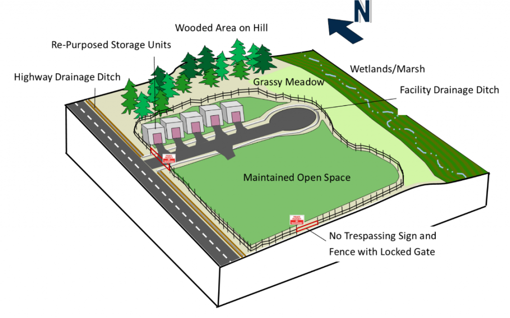
Source: ITRC ISM Update Team, 2020.
Historical site use. Historically, the industrial site was a redistribution center for a paint manufacturer (Figure 3-12b). Large truck shipments came from manufacturing centers across the country, and their products were off loaded, stored, and then loaded back onto trucks for local and regional redistribution to commercial outlets. No manufacturing or repackaging occurred on the property; products were only off loaded, stored, and then loaded and shipped. However, the product was sometimes damaged, and along with other facility trash, it was dumped in a small, private landfill on the southeast corner of the property (Figure 3-12b).
In addition to the storage units that are still standing and in use today, the site also had an administrative building with an adjacent employee parking lot and a redistribution warehouse with an indoor handling area as well as loading docks. Two roadways connected the areas on the site: the main site road that started at the western (main) entrance gate off the highway and extended to the turnaround area on the eastern part of the property, and a secondary access road by the former employee entrance on the southern property boundary. The main access road has drainage ditches on either side of it as well as around the turnaround area. The sloping topography from north to south facilitates drainage and overland transport of soil fines, so although these ditches only hold water for brief periods after rain events, the main road ditch system did and continues to require regular maintenance to maintain open drainage. The secondary road leading to the loading docks and the employee parking lot did not need drainage when the facility was operating, but water has been seen to collect in this part of the property in recent years.
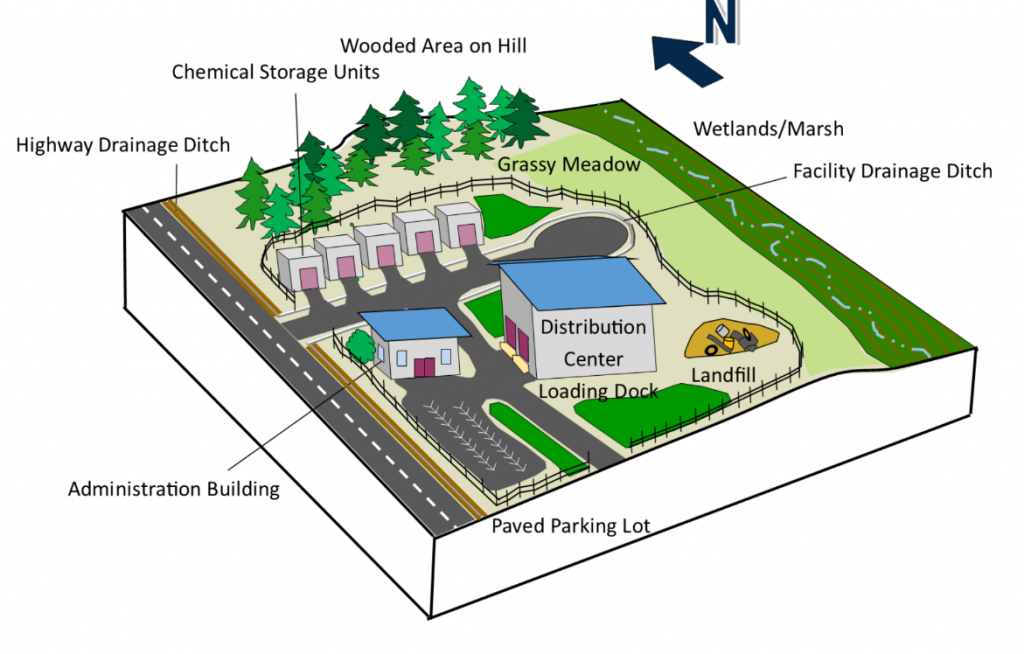
Source: ITRC ISM Update Team, 2020.
DQOs. The following example shows one possible route a site investigation could take. The approach presented here is not intended to portray the only approach to take – rather, it will walk the reader through the logic that the DQO process could take to illustrate how ISM sampling can meet more than one end-use objective.
DQO step 1: problem formulation. Preliminary problem formulation requires the consideration of a sequence of steps:
- identification of potential primary source areas/release mechanisms
- identification of potential secondary source areas/release mechanisms
- identification of media that could be impacted by such a release/migration (exposure media)
- identification of receptors, both human and ecological, that could come into contact with these contaminated media (potentially completed pathway)
- First, generate the preliminary CSM and potentially complete exposure pathways to establish DUs.
- Primary source areas/release mechanisms. Based on past site usage, it has been agreed that there are two potential primary source/release areas: one, the portion of the secondary road in the vicinity of the former loading/unloading docks where material could have been spilled during loading/unloading (Figure 3-13a, DUs 1 through 5), and two, the former landfill where wastes of various kinds were buried and could infiltrate/percolate the soil column (Figure 3-13a, DUs 6 through 13).
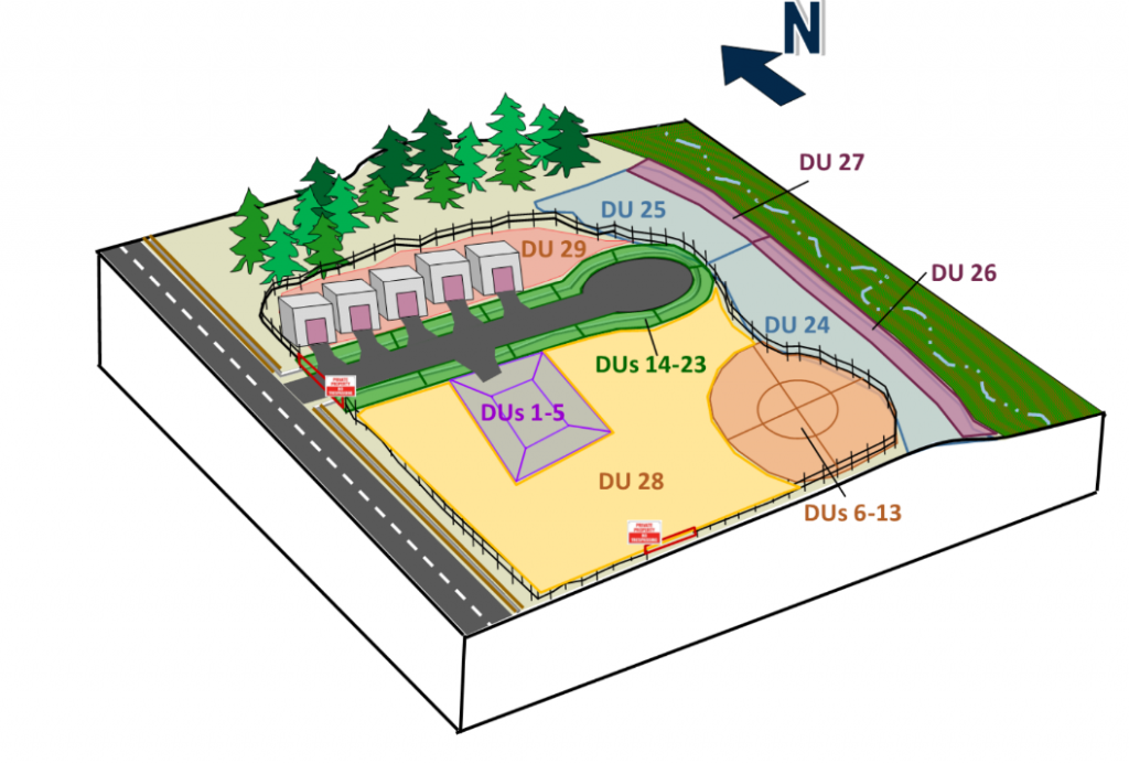
Source: ITRC ISM Update Team, 2020.
- Secondary source areas/release mechanisms. The primary release mechanisms in both instances leads to contaminated soil as a secondary source. These contaminated soils can, via a secondary release mechanism, release COPCs through overland transport of fines and particulate (horizontal transport), infiltration/percolation (vertical transport), and dust and/or volatile emissions (horizontal transport). These secondary source areas then become exposure media.
- Exposure media. Although some shaping and grading of the site has occurred over the years to direct rainwater to drainage ditches, the topography of the site is essentially level. For this reason, the drainage ditches along the main roadway and the turning area are considered to be potentially impacted. However, due to the hill on the northern border of the property and the wetland on the eastern border, COPCs could also potentially move westward via overland transport and infiltrate/percolate. As a result of this and the proximity of the former landfill to the grassy meadow and wetland, soils/sediments in these areas could impact media differently from the northern shore area. Based on the topography of the site, it is expected that dust and/or volatile emissions could result in widespread and more diffuse impacts. All these successive layers of systematic planning are presented in the final figure for each group of site receptors.
- Human receptors. Four human receptors have been identified: industrial/commercial workers who could contact soils anywhere within the property boundaries, as well as the ditches; construction workers who would encounter soils in the maintained portion of the property south of the main road; trespassers who would encounter soils in the grassy meadow east of the property; and trespassers who would encounter sediments along the shoreline the wetlands east of the property (Figure 3-13b).
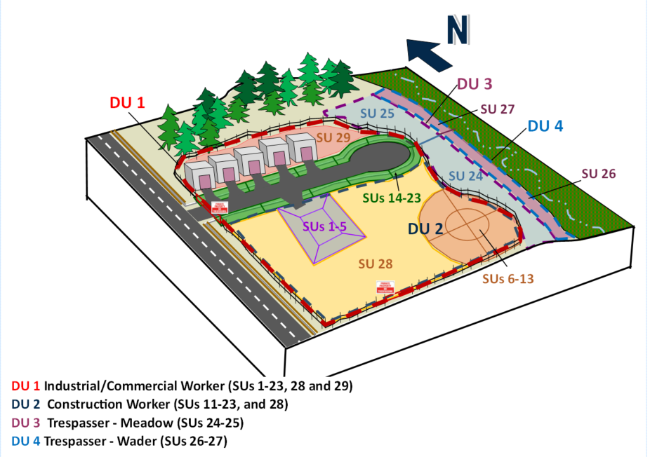
Source: ITRC ISM Update Team, 2020.
- Ecological receptors. Two categories of ecological receptors have been identified: terrestrial receptors that would use the grassy meadow, and two aquatic receptors that would use the aquatic habitat. A review of representative receptor categories for the site indicates that all categories of representative receptors would utilize the entire area of the two identified habitats east of the property (Figure 3-11c).
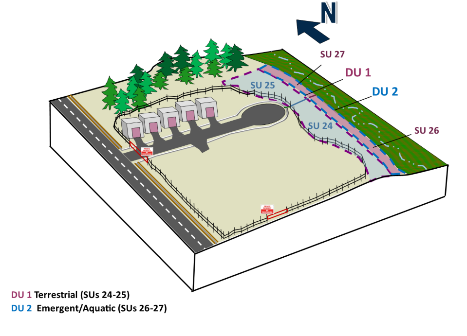
Source: ITRC ISM Update Team, 2020.
All these components of problem formulation can be summarized in a CSM (see Figure 3-14a and Figure 3-14b).
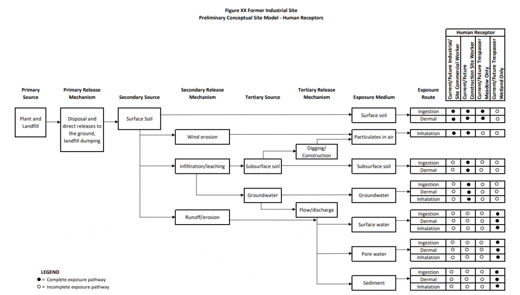
Source: ITRC ISM Update Team, 2020.
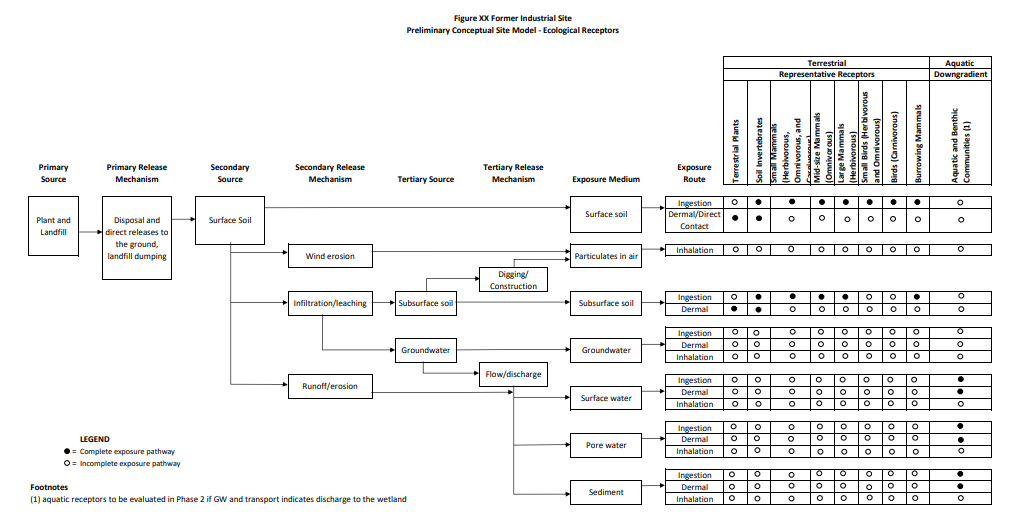
Source: ITRC ISM Update Team, 2020.
DQO step 2: identifying study goals.Repurposing this site cannot occur until the site investigation questions are answered. Using the CSM as the starting point for systematic planning and DU design, the project team needs to identify study goals to ensure the data collection will generate data of sufficient quality and quantity to achieve the study goals.
In this case, three study goals have been identified:
- Has the N&E of site-related releases been fully characterized?
- If human or ecological receptors are exposed to site-related COPCs via contaminated soil/sediment, are they exposed at levels that present risk?
- Ultimately, if risk is present, what mitigation measures might be needed?
It is not always possible to plan the full timeline of the investigation/remediation, but consideration should be given to the entire continuum of activities through the involvement of the appropriate technical specialists who will be involved over the duration of the project. Often, minor modifications early in the development of sampling and analysis plans/QAPPs can save time and money at a later stage of the project by removing the need to remobilize to collect similar but not identical data. This planning can contribute data to both the investigation/evaluation phase as well as the remedial measures phase.
DQO step 3: identifying information inputs. As the sampling and analysis plan/QAPP is developed, the project team should evaluate what specific information is needed to evaluate the study goals. In particular, when developing an ISM sampling approach, they should consider the specific purpose of each piece of data collected. ISM samples can be collected from DUs or SUs, but the assignment of an ISM sampling area to one category or the other depends on the use to which it will be put.
Recall from earlier text that both SUs and DUs are separately collected samples, with SUs being subdivisions of DUs. Simply put, if an ISM sample is used as a stand-alone sample to make a decision, it is a DU; if the ISM sample is used in conjunction with another ISM sample(s) to make a decision, it is an SU.
In the example with three study goals (DQO step 2), rather than trying to develop an integrated plan that lays out all SUs and DUs simultaneously, it is strongly advised that the sampling requirements of each study goal be worked out systematically by each technical specialty within the project team, then the team can integrate the various sampling needs into one sampling plan. As will become apparent in this example, systematic planning can define both SUs and DUs and allows for the contingency that a DU for one study goal may become an SU for another study goal.
DQO step 4: define study boundaries. The primary questions to answer when defining study boundaries are (1) “Where is the contamination located, and are there spatial patterns?”, and (2) “What is the average concentration that needs to be defined for each study goal?” Answering these questions requires translating the components of the CSM into a sampling plan where the number, location, and dimensions of SUs and DUs can achieve the study goals (DQO step 2) and support site decisions.
- Study boundaries related to estimating average soil concentrations. Two types of average soil concentrations are needed to achieve the study goals for the former industrial site: average concentrations to define source areas and average concentrations to define exposure to human and ecological receptors. To collect meaningful data for source areas, the project team can use historical site information, aerial photographs, satellite imagery, and other historical sources to help define the areas that need to be investigated. For exposure estimates, the CSM must be developed (DQO step 1) and integrated with the resource/habitat characteristics on and within the potentially impacted site.
- Source area DUs. Figure 3-13a shows both primary and secondary source DUs, with primary source area N&E DUs 1 through 5 near the former loading dock area and N&E DUs 6 through 13 in the former landfill area. Both sets have a central DU placed where the highest levels of potential releases may be, with the DUs around it determining if the central source area was targeted correctly and indicating how much the original release may have spread.
For this property, secondary source areas are adjacent but more spread out – for example, the drainage ditches (N&E DUs 14 through 23), the grassy meadow (N&E DUs 24 and 25), and the wetlands (N&E DUs 26 and 27) (Figure 3-13a). The drainage ditches were divided into 10 DUs to allow for various transport mechanisms to be evaluated. If the ditches show minimal silting and that concentrations within any particular DU are low, the sampling allows the option of deciding to only clean out silted in areas in a subset of the DUs. Along similar lines, each habitat zone has two DUs to allow the area near the landfill to be compared to the portion of the habitat zone more distant from the landfill, which should provide insights into the fate and transport from the former landfill.
- Exposure area DUs for human receptors (HH DUs). Figure 3-13b shows DUs associated with areas where humans may reasonably expect to come into contact with site soils and sediment on or adjacent to the site currently or in the future.
Disregarding the SUs in these figures. Each human receptor has a distinct exposure DU based on (1) an ongoing activity (industrial/commercial worker over the entire property, human health (HH) DU1 in the figure outlined in red dashed lines); (2) a reasonably anticipated future role (construction worker in the portion of the property south of the main access road, HH DU2 outlined in blue dashed lines); or (3) a transient current or future trespasser exposure in the grassy meadow (shown as HH DU3 outlined in dashed purple lines) and the wetland shoreline (HH DU4 outlined in dashed light blue lines).
- Exposure DUs for ecological receptors (Eco DUs). Figure 3-13c shows DUs associated with areas where ecological receptors may reasonably expect to come into contact with soils and sediment on or adjacent to the site currently or in the future.
For this particular site, the ecological receptors are limited because of the limited habitat. The maintained grassy area with the property fence is not considered an ecological resource because it is artificially maintained, however, the areas east of the site are. The grassy meadow that is used to assess potential exposure to terrestrial receptors, Eco DU1 (outlined in dashed purple lines), is the same as HH DU3 for the grassy meadow trespasser. Similarly, Eco DU2 (outlined in dashed light blue lines) is the same as HH DU4.
- Study boundaries related to evaluating the N&E of contamination. N&E must be evaluated both vertically and horizontally.
- Evaluation of the vertical extent of contamination. Three major factors should be considered when considering the vertical extent of contamination: What was the nature of the COPCs? At what depth were they introduced? What depth horizons are required to evaluate exposure for current or reasonably anticipated future receptors? Knowing the nature of the COPCs will allow advance evaluation of the fate and transport of the release. Surface releases may not migrate through the soil column, while containers buried at 10 ft below ground surface that leak starting at depths of 10 ft present a very different scenario for assessing vertical migration. Lastly, along with these two considerations, the depth horizons that need to be sampled to evaluate exposure to human and ecological receptors must also be integrated.
In the secondary source areas (drainage ditch, grassy meadow, and wetland shoreline), spills where potential contamination is expected to be less than in the primary release areas might have you deciding to limit sampling to only surficial soils for N&E and only sampling deeper if the exposure horizons warrant it or surficial soils show elevated levels of site-related COPCs.
- Evaluation of the lateral extent of contamination. Lateral extent is handled immediately around the source area DUs with a peripheral ring of DUs that serves two purposes: (1) help to bound the source area, particularly if the placement of the source area had some uncertainty associated with it, and (2) provide insights into possible lateral migration.
- Evaluation for the presence of subareas of elevated contamination. Vertical soil horizons and multiple adjacent DUs commensurate in size with the site history and suspected release allow the team to address the presence of subareas of elevated contamination. Large DUs may help the team assess exposure but run the risk of overlooking subareas where COPC concentrations could be elevated. The needs of N&E DUs and exposure must be balanced. If smaller areas are needed to delineate N&E, they can be reassigned to SUs for the evaluation of exposure; an area-weighted average can then be used to create an EPC for the purposes of evaluating risk.
Integrating the sampling needs for N&E with exposure. Once sampling plans for each study goal are worked out, they should be integrated into one single project sampling plan, and the overlap – as well as the differences – between each plan should be understood by the project team. Minor changes in sampling can take data that are useful for only one study goal and make them useful for two or more other goals. Care should always be taken to recognize when a DU for one study goal can serve as an SU for another study goal.
Looking at the more straightforward ecological exposure scenario (Figure 3-13c) first, only two Eco DUs are defined, one for the grassy meadow and one for the wetland shoreline. However, each of these DUs contains two SUs that were designated N&E DUs (Figure 3-13a). The ecological exposure needs to be evaluated for the entire grassy meadow and the entire shoreline, but these zones were divided into two N&E DUs to examine the effect the landfill might have had on environmental media adjacent to the site. If elevated concentrations are noted in N&E DU26 compared to N&E DU27, it would confirm that transport had occurred off the site. However, within the risk context, the area-weighted average of SU26 and SU27 may show no risk is present. At this stage, the project team would need to evaluate this within the context of the project goals to decide how to proceed.
Turning to the human health exposures (Figure 3-13b), identical logic would be applied to trespassers who use the Figure 3-13a N&E DUs as SUs within the exposure scenario to derive an EPC using an area-weighted average. The EPCs for the two receptors within the property boundaries would also be arrived at through the use of an area-weighted mean, using the N&E DUs as exposure SUs where the industrial/commercial worker includes SUs 1 through 23 as well as 28 and 29 in the derivation of the area-weighted EPC, while the construction worker would include SUs 11 through 23 and 28 in the derivation of the area-weighted EPC. A further refinement could include accounting for the frequency and duration a receptor spends within a particular SU, which could yield an EPC that reflects both spatial and temporal exposure.
Similarly, for the off-site human receptors, the meadow trespasser exposure DU is comprised of SUs 24 and 25 (Figure 3-13b), and the wader trespasser exposure DU is comprised of SUs 26 and 27.
3.2 Statistical Concepts and Applications in ISM Projects
The purpose of this section is to introduce key statistical concepts that are relevant to both the sampling design and analysis of ISM data. Many of these concepts are not unique to ISM and will be familiar to analysts for their use in other contexts. While this section is not intended to serve as a comprehensive guidance on environmental statistics, it does address many of the common questions that practitioners will likely have. Citations and hyperlinks are provided to guidance documents, white papers, peer-reviewed literature, and calculation tools to supplement the information presented here. In addition, several hypothetical examples with ISM data sets are included.
3.2.1 Why use statistics?
Statistical concepts have long been used to guide decisions involving both environmental sampling and inferences based on sample results. Regulatory guidance and quantitative tools facilitate the application of statistics methods that are transparent, objective, and defensible given site conditions (USEPA 2015). Statistical methods can be used to quantify uncertainty and express the level of confidence in estimates of exposure and risk – in turn, this consistency and reproducibility promotes consensus among parties with competing interests. Moreover, including statistical concepts during project planning prior to data collection or as a component of a tiered approach (such as adaptive sampling) can help stakeholders and project teams make scientifically defensible decisions for site investigations. Investigations guided by statistics are also more likely to result in cost-effective outcomes that achieve goals protective of human health and the environment.
This section describes the application of classic inferential statistical analysis methods to ISM data, assuming the sampling design yields a representative sample consistent with a study’s objectives. A discussion of statistical concepts that inform the collection of physically representative samples (increment mass given the properties of the medium) and explicit accounting of sources of measurement errors is beyond the scope of this section.
3.2.2 Confidence intervals of the DU mean
Statistics are often used to calculate an upper bound estimate of the AM contaminant concentration of a DU, referred as a UCL of the DU mean. While the “true” population mean of a DU cannot be measured exactly, it can be estimated from an ISM sample with some specified tolerance for uncertainty. For environmental investigations, we are typically interested in choosing a method that yields a UCL greater than or equal to the population mean 95% of the time, which is why we call it the 95% UCL. This guidance explains how ISM introduces procedures to cost-effectively reduce sources of measurement errors in the field and the laboratory. This section discusses key statistics concepts and procedures that can be applied to both inform the sampling design and compute a reliable 95% UCL.
Typically, only a small portion of a DU is sampled. A statistician would refer to the set of concentrations reported from the environmental (or soil) samples randomly collected from the same DU as a sample. A variety of summary statistics can be computed from the sample, such as the set of environmental sample concentrations. The sample mean is the numerical mean of the concentrations and is often represented as x bar, or x. The sample mean estimates the true DU mean, which statisticians refer to as the population mean and often denote with the Greek symbol µ. It is very unlikely that the sample mean ( x ) and population mean (µ) will be exactly equal. For any single investigation, may be smaller or larger than µ. In general, we want to choose sampling designs that yield rigorous statistics. One way to achieve this would be to repeat the same investigation of a DU many times, generating a sample mean ( x ) each time some of the sample means would be less than the population mean, and some would be greater, but the mean x would provide a reliable estimate of µ. Since it is impractical to resample a DU many times, we can rely on statistics instead. Three key statistics concepts tell us important facts about the sample mean generated from any single ISM investigation:
- Random sampling yields unbiased parameter estimates. If a random sampling design is used, the sample mean will be unbiased, which means that, on average, x equals µ. Statisticians often express this equality by stating the average difference ( x – µ) = 0. This desirable property is true for any sampling design that applies random sampling, including ISM.
- The sample mean from one investigation is more likely to underestimate than overestimate the population mean. The chance that any one sample mean underestimates the population mean (that is, ( x – µ) < 0) depends on the shape of the probability distribution of the mean concentrations of the concentrations. If the PD is symmetric (or normal), there is an equal probability that x will underestimate or overestimate µ. If the distribution is skewed, the probability is unequal and depends on the direction and magnitude of the skewness. Most environmental datasets exhibit positive skew, which means that when they are plotted as a histogram, they have a tail that extends to the right. Under this condition, there is a greater probability that the sample mean underestimates (rather than overestimates) the mean (that is, ( x – µ) < 0 is more probable than ( x – µ) > 0).
- A key advantage of ISM over discrete (grab) sampling, which both simplifies the statistics and helps generate reliable results, is that it invokes the central limit theorem (CLT). Each replicate of an ISM sample can be thought of as an independent estimate of x. If an ISM sample includes three replicates (r = 3), each generated with 30 increments (n = 30), we will have three different values from which we can compute summary statistics, such as the AM and SD. It can be helpful to think of the mean of all DU replicates x as the mean of the means or the grand mean. Importantly, the distribution of x values differ from the distribution of concentrations for each increment (n). Specifically, the distribution of x exhibits three key properties: (1) the shape of the distribution is more symmetric (less skewed); (2) the SD of x is lower; and (3) the grand mean yields an unbiased estimate of µ (as described above). Statisticians refer to the CLT when talking about the distribution of x. The CLT tells us that as the sample size (n) increases, the shape of the distribution of x tends toward a normal distribution, even if the distribution of increments is quite skewed. The fact that the distribution of x approximates a normal distribution and that this approximation improves with increasing sample size (n) has important implications for 95% UCL calculations, as discussed further below. ISM basically incorporates superior coverage and sample processing steps to create a physical realization of the CLT.
In risk assessment, an EPC is typically based on a 95% UCL so that risk-based decisions are protective of human health and the environment (USEPA 2002). The purpose of a 95% UCL calculation is to provide an estimate of µ from a single investigation, such that we are unlikely to underestimate long-term average exposure. With statistical methods, we can express the likelihood of under- and overestimation by calculating a confidence interval(CI)for a population parameter. Each CI is defined by a lower confidence limit (LCL) and UCL. There are two relevant properties of a CI that we can specify: (1) the probability that the CI contains the population parameter and (2) whether the CI is one- or two-sided. A one-sided CI is one in which the population parameter is permitted to fall on one side of the CI, either below the LCL or above the 95% UCL but not both. A two-sided CI is said to contain the parameter with a certain probability, but the parameter may be either less than the LCL or greater than the 95% UCL. A 95% UCL is one-sided, such that it has a 95% chance of being greater than or equal to µ. This convention addresses the risk assessment goal of erring on the side of protectiveness of human health and the environment.
Using numerical simulation studies and statistics theory, we can evaluate the performance of different 95% UCL methods under varying site conditions. USEPA, for example, has conducted extensive simulations to evaluate the performance of 95% UCL methods calculated with the software tool ProUCL (USEPA 2015), and ITRC has also conducted extensive simulations to understand the performance of 95% UCL methods applied to ISM datasets. Two key performance metrics are 95% UCL coverage and CI width:
- Statisticians use the term coverage to refer to the frequency with which a 95% UCL equals or exceeds µ. A 95% UCL is intended to equal or exceed µ 95% of the time (and fail to exceed µ 5% of the time) if the same sampling design was repeatedly applied to a DU. Therefore, one goal of a 95% UCL method is to achieve a coverage of 95%. Different 95% UCL methods can yield different coverage probabilities, so one decision criteria for 95% UCL method selection is to determine if the method yields reliable (at least 95%) coverage, across a wide range of site conditions. An incorrectly chosen calculation method may provide coverage that is less than 95% (say, 85% or 90%).
- In addition to yielding different coverage probabilities, 95% UCL methods can yield different sizes (or widths) of CIs. The width of the CI is a measure of the uncertainty of the estimate of the DU mean(NIST, 2019). The larger the CI width, the larger the uncertainty. In general, the width of the CI increases as the variability of the data and required level of confidence increases. In addition, different 95% UCL methods can yield different 95% UCLs when applied to the same summary statistics. If two 95% UCL methods achieve the same coverage, the method that yields a narrower CI (that is, lower than 95% UCL) is preferred (USEPA 2015).
Therefore, to effectively choose between 95% UCL methods, we need to understand the performance of each method under the specific conditions of interest and balance the dual objectives of 95% UCL coverage and CI width. Summaries from simulation studies conducted with ISM samples are presented below to help guide the selection of 95% UCL methods.
3.2.3 Illustration of the CLT using Pb data from the Becker study
The next series of figures is a graphical representation of the CLT. The data used to construct the CLT graphs were taken from the Becker study described in Section 2.2.2. The dataset consists of the 129 Pb results making up one of the four contaminated arrays evaluated for the study (Note that the Becker study evaluated four arrays, one of which is depicted in Figure 2-3a). Figure 3-15 plots a lognormal distribution fit to the dataset consisting of 129 individual Pb sample results. The 129 results range from a low of 48 to a high of 22,000-mg/kg Pb. The distribution is skewed to the right by the presence of a few extremely high results. Approximately 50% of the results are less than 2,400 mg/kg (as indicated by the median, equivalent to the geometric mean for lognormal distributions).
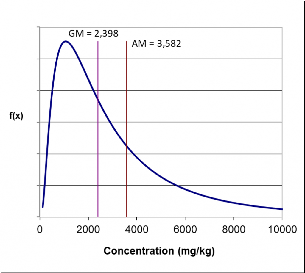
Source: ITRC ISM-1 Team, 2012.
The CLT states that, for any random variable X with a (population) mean of µ and finite variance σ2, the (sample) mean of a set of k independent replicates of X will approach a normal distribution with variance σ2/k as k increases. In other words, regardless of whether or not X is normally distributed, when the numerical mean is calculated from a sufficiently large number of k replicates, the numerical mean of the replicates will be approximately normally distributed, and the variance of the mean will be equal to the variance of the replicates (σ2) divided by k. Also, assuming the sampling design involves collecting the samples at random, the sample mean yields an unbiased estimate of the population mean.
For the purposes of illustrating the CLT concept, we can study how the distribution of sample means changes when we repeat many sampling events at a site for which the distribution of Pb concentrations in soil is described by a lognormal with a population mean (µ) 3,582-mg Pb/kg soil and population SD (σ) of 3,976 mg/kg. Each ISM sampling event generates a replicate r consisting of n increments. With a numerical simulation, we can repeat the exact same sampling program (n, r), drawing random samples from the lognormal (µ, σ) many thousands of times, each time recalculating the sample mean from the r replicate results.
If we repeat the sampling program 150 times (r = 150), we generate 150 sample means. Through simulation, we can examine the following types of questions: (1) How does the distribution shape change as n increases (at what point is the distribution of means approximately normal)? (2) Does the mean of the 150 sample means (the grand mean) change as n increases? (3) Does the SD of 150 replicate means change as n increases?
For this example, the simulation is repeated three times using n = 5, 15, and 30, each with r = 150. The resulting distribution of sample means is illustrated in Figure 3-16 and summarized in Table 3-2 below. We can now provide answers to the questions outlined above:
- It turns out that the greatest effect of changing n is on the distribution shape. The shape of the distribution becomes more symmetric and approaches a normal distribution as n increases. This is a key concept of the CLT.
- According to the CLT, the grand mean should approximate the population mean. In this example, the population mean is 3,582 mg/kg, and the grand means for the three simulations are 3,438; 3,842; and 3,672 mg/kg (see Table 3-2).
- The SD of the set of r = 150 sample means depends on the choice of n. Specifically, the SD of the sample means is approximately proportional to the inverse of the square root of n.
In practice, an ISM investigation will generate very few datasets – for example, r = 1 to 3, and n = 30, from which we calculate one set of summary statistics for the sample mean (such as mean, SD). Therefore, with only 1 to 3 estimates of the population mean, we cannot rigorously explore the shape of the distribution of sample means with the usual goodness-of-fit statistics and data visualization methods. Note that at least n = 30 increments are typically used to prepare ISM samples when it is reasonable to assume there is mild to moderate heterogeneity (see Section 3.2.4.2 and Table 3-3). The extent of heterogeneity is a result of the dispersion of the data and the shape of the distribution.
Source: ITRC ISM Update Team, 2020.
Table 3-2. Summary statistics for sample means generated by simulating ISM sampling events with r = 150 replicates and n = 5, 15, and 30 increments.
Source: ITRC ISM Update Team 2020 based on data from Becker, 2005.
| Statistic | Population | Scenario A | Scenario B | Scenario C |
| Sample Size | 129 | n = 5, r = 150 | n = 15, r = 150 | n = 30, r = 150 |
| Minimum | 48 | 906 | 1,896 | 2,063 |
| Maximum | 22,000 | 9,990 | 7,216 | 6,990 |
| Range (Max – Min) | 21,952 | 9,084 | 5,320 | 4,927 |
| Mean | 3,582 | 3,438 | 3,842 | 3,672 |
| SD | 3,976 | 1,616 | 1,037 | 808 |
| CV | 1.1 | 0.47 | 0.27 | 0.22 |
| RSD | 111% | 47% | 27% | 22% |
| Distribution Based on Goodness-of-Fit Statistics | Lognormal | Lognormal | Lognormal or Gamma | Normal |
| 95% UCL | Not applicable | Chebyshev = 4,012 | App. gamma = 3,986 | Student’s-t = 3,782 |
Notes: n = number of observations per event; r = number of repeated sampling events; CV = coefficient of variation = SD/mean; RSD = relative standard deviation = CV x 100%
3.2.4 95% UCLs
ISM samples provide estimates of mean concentrations, but many factors can cause an ISM sample’s concentration to deviate from the true DU mean concentration. Under some circumstances, those deviations can be large. In one project, BaP concentrations greater than 466 µg/kg triggered DU cleanup. The first ISM sample had concentrations well below that, but additional replicate ISM samples were well above, for example, the first ISM sample = 380, the second = 1,100, and the third = 1,400 µg/kg BaP.
| Severe underestimation by a single ISM sample is possible, leading to decision errors unless precautions are taken. Those precautions include replicate ISM samples and the use of 95% UCLs in decision-making. |
In theory, all 95% UCL methods that are applied to discrete sampling results can also be applied to ISM. However, in practice, the options for 95% UCL methods with ISM are constrained because the small number of replicates (r = 3) precludes a rigorous evaluation of distribution shape and application of bootstrap resampling methods when distributions are not consistent with normal, gamma, or lognormal distributions.
Goodness-of-fit evaluations that inform the shape of the distribution require at least 8 to 10 observations from a dataset, possibly more if the data are highly censored (meaning they include non-detects) (USEPA 2016). Typical ISM sampling designs include fewer than 8 to 10 replicates – in fact, three replicates are often used to estimate the SD of sample means. Such small sample sizes limit the options for statistical analysis of ISM data to two methods for 95% UCLs calculations: Student’s-t and Chebyshev. The formulas for these two methods are presented below. Other 95% UCL calculation methods may be explore for larger sample sizes (e.g., r ≥ 8 to 10) (USEPA 2016).
The Student’s-t 95% UCL is restricted to datasets that follow approximately normal distributions. For ISM, physical averaging based on increased sample volume effectively reduces the variance in the underlying distribution of increments, but it cannot guarantee that the distribution is normal – on the contrary, it is expected that some degree of positive skewness will still occur for most sites. It would be incorrect to state that the CLT is always going to sufficiently normalize the distribution of replicate means to support an assumption of normality (USEPA 2016). Therefore, the key assumption for the approximate normality required to select the 95% t-UCL should be considered carefully. In cases where the underlying distribution for increment-sized soil masses is highly skewed (Figure 3-16), 30 increments may not be enough to normalize the distribution of replicate means. In such cases, the Student’s-t 95% UCL may not provide the desired statistical confidence since it will have a greater than 5% chance of underestimating the population mean. Recalling the discussion of 95% UCL coverage associated with Figure 3-16, another way to say this is that the 95% t-UCL would not actually provide 95% coverage of the true mean. With a highly skewed underlying population, the 95% t-UCL might only cover the true mean 80% or 90% of the time. Of course, since the population mean is unknown, in practice, we cannot calculate or even conduct a simulation study to estimate the coverage for a site. Therefore, we rely on simulation studies of a range of different conditions with known population parameters in order to guide the selection of 95% UCL methods based on properties of the ISM dataset.
Figure 3-17 illustrates the CLT for n = 30 ISM samples and for underlying distributions (the individual increments represented by the pink curves) having various level of skew (right-hand tail). Skewness increases as CV increases from 0.5 to 3.0, left to right. Between a CV of 1 and 2, the skewness of the underlying population becomes too great for n = 30 to normalize the distribution of replicate means (blue curves).
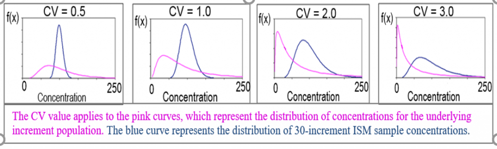
Source: ITRC, 2017, ITRC Webinar: Soil Sampling and Decision Making Using Incremental Sampling Methodology – Part 1, Module 4 (Statistics).
Asymmetry in the distribution of means with CV > 1 indicates the assumption of normality is not supported. If the population of replicate means is not near-normal, the 95% t-UCL will likely not provide adequate coverage for the DU mean. As noted in the discussion of the CLT above, one option to improve the symmetry of the distribution of replicate means is to increase the number of increments per ISM sample replicate. As shown in Figure 3-17, the normalizing effect of the CLT is better when n is larger (n = 30 versus 15 or 5). For this example, the CV of the underlying distribution of increments was 1.1, but no single rule regarding sample size will apply universally because the key is the shape and spread of the underlying distribution of increments.
The Chebyshev method is a viable option to calculate the 95% UCL because it reduces the chance the 95% UCL will underestimate the population mean. The Chebyshev 95% UCL is a nonparametric 95% UCL, which means that it can be used when the data distribution is unknown or is not normal. In many cases, it can achieve the desired 95% coverage even with r = 3 replicates and n = 30 increments. Reducing the skew in the distribution of means by increasing n will improve the performance of all 95% UCL methods, including the Chebyshev. The Chebyshev is considered to be a conservative estimate of the 95% UCL because it generally achieves or exceeds the desired coverage rates, even for non-normal distributions. The Chebyshev is able to achieve the coverage for skewed distributions because the Chebyshev 95% UCL is higher than the 95% t-UCL. In other words, for a given (1 – α) confidence level, the CI width for a Chebyshev 95% UCL is greater than for a 95% t-UCL, given the same ISM dataset (r, mean, SD). The implication for decision errors is that the Chebyshev 95% UCL is less likely to underestimate the true mean and lead to an erroneous conclusion that a DU is “clean” when in fact it is “dirty.”
The initial ITRC ISM document provides recommendations on the selection of 95% UCL methods, given properties of the site and ISM summary statistics. At that time, other than at military ranges, practitioners had little experience with applying ISM to the more common types of sites, so the key observations and recommendations might not have been applicable:
- If the underlying population distribution is only mild to moderately skewed, the default number of increments per DU/ISM field sample required to normalize the ISM data is at least 30 (refer back to Section 3.2.4.2). As a rule of thumb, if the population CV < 1.5, the distribution is likely relatively normal or mildly skewed; if CV = 1.5 to 3, the distribution is moderately skewed; if CV > 3, the distribution is very skewed.
- It is possible that fewer increments per ISM sample will suffice, but data should be collected to demonstrate this statistically. These data are efficiently collected as part of a pilot study, but a pilot study is generally cost-effective only for large projects with many DUs of the same type. For smaller projects, it is more efficient to simply use the default.
- It is possible for DU heterogeneity to be higher than expected, so 30 increments will be too few, and replicate ISM samples will not agree as well as expected.
- As the underlying DU population becomes more skewed, normalization by increasing the number of increments (see discussion of the CLT in Section 3.2.3) becomes less effective. This was illustrated by computer simulations for 30 increments.
- Recall that the same normalization occurred for the Pb mean data in Section 3.2.4.2. The skewed underlying distribution of 129 Pb concentration data (variability of 111% RSD, which is equivalent to a CV of 1.11, refer to Table 3-3) was fully normalized by 30 field samples per sampling event, which is equivalent to 30 increments per ISM sample.
3.2.4.1 Calculating ISM 95% UCLs and a word of caution about ProUCL
The equations for Student’s-t and Chebyshev 95% UCLs are easily programmed into an Excel spreadsheet file (see ISM 95% UCL Calculator). The methods will yield two different 95% UCL values, prompting a decision as to which of the two to use. Because ISM projects rarely measure the underlying distribution of the increments (that is, analyze at least 10 individual increments and run statistical analysis on the dataset), the CV of the underlying distribution can be estimated from the SD and the number of replicates, and the calculations can be built into a spreadsheet. Such an ISM 95% UCL calculator was built by the first ISM Team and has been updated since then with an improved modeling procedure. The calculator has several benefits:
- The user only has to enter the results of three to six replicate field samples, as well as the number of increments per sample.
- The ISM 95% UCL spreadsheet calculates both the Student’s-t and Chebyshev 95% UCLs.
- The spreadsheet recommends which 95% UCL should be used.
Many practitioners are familiar with using ProUCL to obtain 95% UCLs for discrete datasets (USEPA 2015). With the release of ProUCL 5.1, ProUCL has been modified to allow calculation of UCLs for datasets with only three sample results. However, results using ProUCL should be interpreted carefully:
- ProUCL may present values from many methods, some of which may lead to an underestimation of the population mean with a greater than 95% frequency. It is important that the selection of a result for a particular dataset is guided by the findings from simulation studies involving small sample sizes and a wide range of types of underlying distributions.
- ProUCL fits the data distribution to several theoretical PDs (normal, lognormal, and gamma distributions). The default assumption is that a dataset fits the theoretical distribution until proven otherwise. However, the statistical tests possess poor power to reject the distribution assumption when the sample sizes are small (r = 3). For example, the underlying distribution of a small dataset may not be normal, but owing to a lack of sensitivity of the statistical test for normality, the assumption of normality will not be rejected (see Section 3.2.3.3). Therefore, ProUCL may recommend the 95% t-UCLs when the sample sizes are small even when that would clearly not be appropriate.
- ProUCL does not perform the calculations to estimate the variability in the underlying increment population and so cannot recommend whether the Student’s-t or Chebyshev 95% UCL is more appropriate.
- The performance of Student’s-t and Chebyshev 95% UCL methods applied to censored ISM data (meaning one or more replicates is qualified as a non-detect) has not been explored. At this time, it is unclear what the coverage probabilities can be expected when non-detects (NDs) are represented by an imputed value (such as half the detection limit).
- For larger sample sizes (r = 8 to 10), the ProUCL software can be used to explore a wider range of 95% UCL methods than the 95% UCL calculator. Note that USEPA guidance on the use of ProUCL 5.1 cautions that at least 10 to 15 observations are needed before relying on bootstrap resampling techniques to estimate the 95% UCL (USEPA 2015).”
3.2.4.2 Formulas for calculating ISM 95% UCLs
Calculation of Student’s-t and Chebyshev 95% UCLs can be readily done using the Excel spreadsheet calculator. Here is the equation for the one-sided (1 – α) Student’s-t 95% UCL:
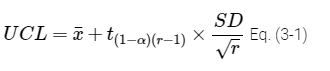
where

For a DU with three replicate ISM samples and a 95% UCL, the equation reduces to the following:

Here is the equation to calculate the one-sided (1-α) 95% UCL using the Chebyshev method:
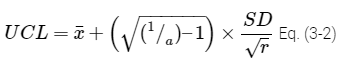
where

For a DU with three replicate ISM samples and a 95% UCL, the Chebyshev equation reduces to the following:
Chebyshev 95%
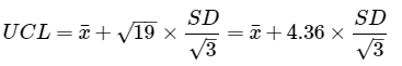
For clarity, SD divided by the square root of the number of replicates is equal to the standard error (SE). Therefore, the SD/sqrt(r) term is equal to the SE of the distribution of the mean of the replicate means.
The probability that a 95% UCL equals or exceeds the population mean of a DU is referred to as the coverage. The desired coverage for a 95% UCL is that, when calculated from an ISM dataset, the value is equal to or greater than the DU mean 95% of the time. Because different 95% UCL methods can yield different coverage probabilities, one criterion for assessing the performance of a method is to examine the coverage probabilities across a wide range of site conditions. For ISM-1 (see Section 1), numerical simulations were conducted to evaluate the coverage probabilities for DUs for which the contaminant distributions exhibited low to high heterogeneity, represented by lognormal distributions with the same AM but different variances. The CV, equal to the ratio of the SD divided by the mean, was selected as the summary statistic to express the dispersion of the distribution. It is important to note that coverage probabilities may vary depending on both the distribution shape and dispersion. Therefore, these simulation results may not apply for all DUs. For cases in which a different positively skewed distribution shape or greater dispersion is suspected, the Chebyshev 95% UCL may be the preferred calculation method because it is more likely to achieve the desired coverage than the Student’s-t 95% UCL.
For ISM-1, the results from the simulations were presented in a table that recommended either a Student’s-t or Chebyshev 95% UCL, depending on the expected degree of dispersion (given by the CV and corresponding geometric SD [GSD]) of the contaminant distribution across increments. A practical limitation of that presentation of findings is that the summary statistics (SD, mean, and CV) from most ISM investigations are based on concentrations measured in replicates (r) rather than individual increments (n). The CV of the increments can be estimated from the CV of replicates by adjusting for skewness of the distribution. For ISM-2, additional numerical simulations were conducted to determine appropriate adjustment factors so that findings from ISM-1 could be applied to statistics based on replicates. Table 3-3 summarizes these findings grouped by the CV of the replicates for r = 3. For example, if an investigation with r = 3 replicates yields a CV of 0.3, the equivalent dispersion for the distribution across increments is a CV in the range 1.5 to 3.0 (medium dispersion), and the Student’s-t 95% UCL would not be expected to yield 95% coverage.
Table 3-3. Likelihood that ISM achieves coverage depending on dispersion (r = 3 replicates).
Source: ITRC ISM Update Team, 2020.
| Degree of Dispersion >> | Low | Medium | High | |
| Dispersion Metric | CV of replicates | < 0.23 | 0.23 < CV < 0.40 | > 0.40 |
| CV of increments (no adjustment) | < 1.26 | 1.26 < CV < 2.19 | > 2.19 | |
| CV of increments (with adjustment) | < 1.5 | 1.5 < CV < 3 | > 3 | |
| 95% UCL Method | Student’s-t | Yes | No | No |
| Chebyshev | Yes | Yes | Maybe | |
Coefficient of variation (CV) = SD/mean. Geometric standard deviation (GSD) = for lognormal distributions.
The difference between Chebyshev and Student’s-t 95% UCLs can sometimes lead to different decisions for a DU. Project teams must balance larger bias associated with the Chebyshev 95% UCL with the smaller coverage of the DU mean associated with the Student’s-t 95% UCL when deciding which method to use. If there is no site knowledge available to support an assumption about the degree of dispersion (that is, low, medium, or high) of increments, then the Chebyshev 95% UCL may be the preferred calculation method because it is more likely to achieve the desired coverage than the Student’s-t 95% UCL.
Another option some practitioners may want to consider is the bootstrap 95% UCL. For a detailed discussion of bootstrap 95% UCLs, refer to the ProUCL technical guidance (USEPA 2015), but note that ProUCL is able to compute bootstrap 95% UCLs as well. To compute bootstrap 95% UCLs requires at least 10 to 15 field replicates for the DU. The bootstrap method involves treating the sample dataset with n observations as the entire environmental population. The population is repeatedly sampled with replacement n times to calculate a sample mean. This process is then repeated many times (say, 1,000) to obtain a distribution of sample means (say, 1,000 sample means). The percentile bootstrap 95% UCL takes the th percentile of the bootstrap means. Like the Chebyshev 95% UCL, bootstrap 95% UCLs have the advantage of being nonparametric, so an assumption of normality is not required. In cases of skewed distributions where the 95% t-UCL is not appropriate, bootstrapping methods may produce a more accurate estimate of the mean concentration that is less conservative than the Chebyshev 95% UCL. However, the percentile bootstrap 95% UCL typically falls short of the desired coverage and may not be appropriate for studies with strict coverage requirements. In addition, bootstrapping is likely to be ineffective for small sample sizes and should not be performed with less than r = 10 to 15 ISM samples.
The bias-corrected accelerated (BCa) bootstrap method is a modification of the percentile bootstrap 95% UCL that attempts to address the issue of insufficient coverage. The BCa 95% UCL corrects for bias in the bootstrapped means by increasing the percentile to be used – for example, if 95% confidence is desired, the BCa method may recommend instead using the 97th percentile of the bootstrap means as the 95% UCL. The recommendation depends on the degree of bias in the dataset. The coverage for the BCa method is improved over the percentile bootstrap 95% UCL, but coverage for the BCa 95% UCL may still fall slightly short of regulatory requirements compared with Chebyshev.
3.2.4.3 Minimizing the CI width in an estimation problem
A large CI width is not desirable when the goal is to confidently estimate the true DU. A common example is deriving the EPC, which uses a 95% UCL to provide an upper bound estimate of the true mean concentration in the receptor’s EU. The 95% UCL is used to avoid underestimating the true mean and thus underestimating risk owing to exposure (USEPA 1992b). The 95% UCL may provide an unreliable estimate of exposure if the dataset is from too few field samples and/or is highly variable (see Section 3.2.2).
Figure 3-17 and the bullets below summarize the factors that affect 95% UCL sizes:
- number of ISM replicates (sample size, n) – the more measurements in the dataset, the smaller the 95% UCL (and CI width)
- degree of variability (range of data values) in the dataset – less variability (a lower SD value) gives a narrower CI width
- desired level of confidence – the higher the desired confidence, the wider the CI width must be (CI width will be narrower for 90% confidence than it is for 95% confidence; at 99% confidence, it will be wider than for 95%)
- data distribution of the population – data distributions (the shape of the data’s histogram) that need to be modeled by a theoretical PD are referred to as parametric methods
For this last bullet, the normal and lognormal distributions may be the most familiar of the different types of PDs. Nonparametric methods do not require the data to be modeled by a particular PD. When applied to the same data or summary statistics, a parametric method (such as the Student’s-t 95% UCL) will generally give CI widths that are narrower than a nonparametric method (such as the Chebyshev 95% UCL). Note that when r = 3, the only difference between the equations for the Student’s-t and Chebyshev 95% UCLs is the value of the multiplier in front of the SD. For a three replicate DU and 95% confidence, the multiplier term is 2.92 for the 95% t-UCL, and 4.36 for the Chebyshev, which is why the Chebyshev 95% UCL will always be higher than the 95% t-UCL.
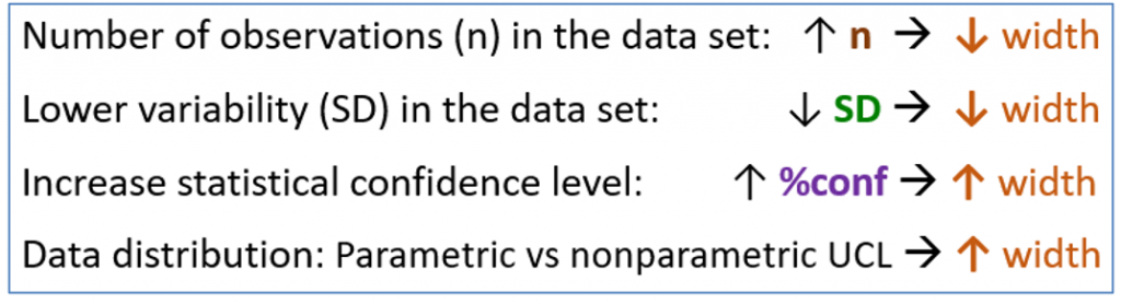
Source: Deana Crumbling, 2020. Used with permission.
Overly large UCLs can be avoided by setting limits on how much uncertainty is tolerable. After coordinating with the risk assessor and stakeholders, the project delivery team might specify the CI width to be no greater than some percentage ( %) of the dataset mean ( ). In other words, the 95% UCL value should be no larger than
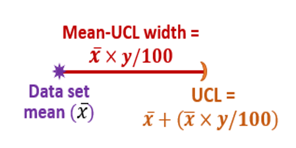
Source: Deana Crumbling, 2020. Used with permission.
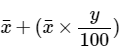
This is illustrated in Figure 3-18. The risk assessor might select the value for y by considering the expected concentration range or the point where the risk calculated from the EPC crosses some important benchmark (the concentrations at which the calculated risk increases from 10-5 to 10-4). More than one y value could be set, depending on what concentrations are found: a wider CI width (and thus a large y) may be tolerated when concentrations are low, but a smaller y may be triggered if DU concentrations turn out to be larger. Setting a limit on the CI width allows project planning to adapt as the data are reported. The calculated DU mean and replicate variability can be used to calculate the 95% UCL. If the calculated width for a DU is greater than desired, additional replicates may be collected to reduce the CI width for that DU (see Section 3.2.2).
The CI width established in Figure 3-18 should be specified in the WP or QAPP. The project team would monitor the data as the data are generated to ensure the objective is being met and take corrective actions if not.
3.2.4.4 Are ISM 95% UCLs valid for risk assessment?
A common question from decision-makers and/or risk assessors is how an ISM 95% UCL compares with a 95% UCL calculated from discrete samples. Some risk assessors believe 95% UCLs based on composite samples are not valid (Mattuck, Blanchet, and Wait 2005). Both ISM and discrete sampling designs can be used to obtain defensible estimates of DU means. However, owing to the CLT, the variability of ISM results tends to be smaller than the variability of discrete sample results, which tend to yield smaller UCLs. ISM sampling designs also tend to result in superior physical site coverage relative to discrete sampling designs. For example, three ISM sample prepared from 30 increments each would be expected to produce a statistical sample that results in similar physical coverage of the site as 90 discrete samples. Also, as explained in Section 2.4.1, soil data variability is influenced by the mass of the analytical subsample. Increasing the analytical mass of an appropriately prepared and subsampled sample (ISM or discrete/grab) will also result in better representation of the sample and ultimate mean coverage from discrete 95% UCL calculations.
The data distribution in Figure 2-8 is largest for the 1-g subsamples, with the distribution narrowing for the 10-g subsamples; the variability in the distribution is smallest for the 100-g subsample set, which means that all the datasets were nearly the same. ProUCL determined that the distribution for the 1-g set was nonparametric and provided a list of eight potential nonparametric 95% UCLs from which to select. The eight 95% UCLs ranged from 2.49 to 4.63, and the 95% UCL that ProUCL recommended had a value of 2.58 nCi/g. The 10-g subsamples had a gamma data distribution, with a recommended 95% UCL of 2.00 nCi/g.
Risk assessors do not normally enquire about the analytical mass when evaluating a dataset, yet in this example, a 10-fold increase in analytical mass produced a 22.5% reduction in the 95% UCL. The same principle influencing the analytical mass applies to the mass of the field sample. Larger field masses reduce the variability of concentration data, which in turn reduces the 95% UCL. An ISM sample is the ultimate field sample mass since, to the best of our technology’s ability, the ISM field sample represents the concentration of the entire DU, and the ISM analytical subsample is managed so that it represents the concentration of the field sample.
3.2.5 Comparisons of 95% UCLs with project decision thresholds
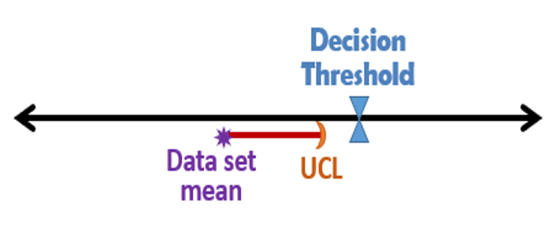
Source: Deana Crumbling, 2020. Used with permission.
A common objective is to determine whether there is sufficient evidence to conclude if the true DU mean concentration is less than some risk-based threshold or other project action limit. As the 95% UCL is the upper end of the CI, the true mean is likely less than the decision threshold if the 95% UCL is below it (Figure 3-19). From the perspective of statistical analysis, the evaluation of compliance with a decision threshold L can be thought of as an example of a one-sample, one-sided hypothesis test (see Section 3.2.5.1). If the UCL is below the threshold, it can be stated with 95% confidence that the true DU mean is also below the decision threshold. In this sense, the 95% UCL of the DU mean controls decision errors arising from measurement uncertainty.
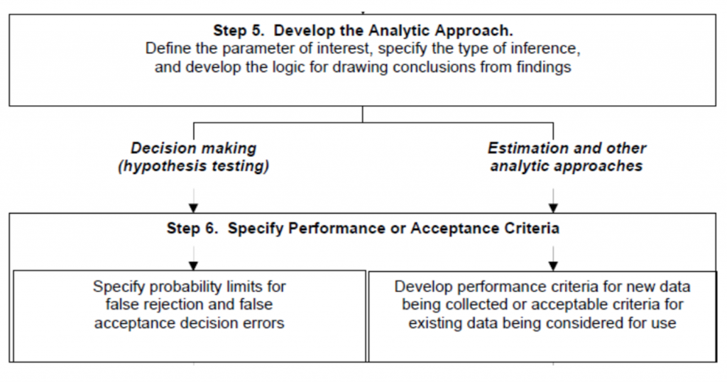
Source: USEPA. 2006b. Guidance on Systematic Planning Using the Data Quality Objectives Process.
Practitioners may be reluctant to tackle steps 5 and 6 of USEPA’s DQO process (Figure 3-20). Abstract and unfamiliar terminology can make the statistical component of this process seem more challenging than it actually is, but Chapter 6 of the update is recommended as a resource for more details than are possible in this document. One of the ways that ISM makes steps 5 and 6 simpler is by making clear that decisions apply to individual DUs, not an entire site all at once (as the wording in the DQO guidance implies). Replacing guidance references to “site” with “DU” brings statistical concepts to a manageable level.
Steps 5 and 6 would also typically entail CIs for estimation problems or hypothesis tests for DUs – for example, the use of a CI to estimate an upper bound concentration for a DU mean (previously discussed in Section 3.2.4) is an example of an estimation problem. Comparing a 95% UCL with a project decision limit or project action limit is essentially equivalent to conducting a one-sample hypothesis test. Comparisons of 95% UCLs with decision thresholds can be used to achieve the same outcome as hypothesis tests and are likely easier to conduct and understand. CIs and statistical hypothesis tests are simply flip sides of the same statistical concepts (USEPA 2006b).
| The easiest way to implement the statistical aspects of the DQO process is by using UCLs. |
3.2.5.1 95% UCLs and hypothesis tests
Hypothesis tests are commonly used to select from one of two mutually exclusive alternative actions or decisions. They require a null or baseline hypothesis (H0) and an alternative hypothesis (H1), with the alternative hypothesis being the condition that needs to be proved. For example, a null hypothesis may be that the DU mean is greater than a compliance level by 10 mg/kg, with an alternative hypothesis that the DU mean is less than or equal to the compliance level plus 10 mg/kg. The null hypothesis is the default condition that data are used to disprove, so a weight of evidence is collected to reject H0 in favor of H1. Often, the failure to reject H0 is an inconclusive result (that is, H0 may or may not be true).
The probability of rejecting H0 (in favor of H1) when H0 is actually true is referred to as the false rejection error, false positive error, or Type I error. The data user’s tolerance for Type I error is usually denoted by the Greek symbol α. It is equivalent to stating the required level of confidence for the hypothesis test (that is, rejecting H0) is 1 – α. The value of alpha often ranges from 0.1 to 0.01, thus the maximum allowable probability for erroneously rejecting H0 is commonly 1% to 10%.
The failure to reject H0 in favor of H1 when H0 is false is referred to as the false acceptance error, false negative error, or Type II error. The tolerance for Type II error is usually denoted by the Greek symbol β, whichrefers to the maximum probability that H0 is false when H0 is not rejected. The quantity 1 – β is referred to as the required power of the hypothesis test, where the power of a hypothesis often ranges from 0.8 to 0.95 and can be viewed as a measure of the sensitivity of the hypothesis test. The larger the power of the test, the more likely the null hypothesis will be rejected when it is false.
More discussion about these relationships can be found in the 2006 G-4 document beginning on page 63 (USEPA 2006b). The tolerance for Type I and Type II error is summarized in Table 3-4.
Table 3-4. Tolerance for Type I and Type II error.
Source: ITRC ISM Update Team, 2020.
| H0 Is True | H0 Is False | |
| Reject H0 (Conclude H0 False) | Type I error, α (false positive) | Correct decision Power, 1 – β |
| Do Not Reject H0 (Conclude H0 True) | Correct decision Confidence level, 1 – α | Type II error, β (false negative) |
Comparing a 95% UCL of the DU mean (µ) with a decision threshold L is equivalent to conducting the following one-sample, one-sided hypothesis test with a Type I error tolerance of 5%:
H0: µ ≥ L, H1: µ < L
This is one-sample hypothesis test because it entails only one population parameter, the DU mean µ. A two-sample hypothesis test would be conducted to compare the DU mean with a background mean. The null hypothesis that the DU is dirty (that is, µ ≥ L) is rejected with 95% confidence when the 95% UCL of the DU mean is less than L. This constitutes what is considered to be an acceptable weight of evidence that the DU is clean. Most cleanup scenarios operate from the assumption that a DU is dirty until proven clean, which is illustrated in Figure 3-21, which is similar to Figure 3-19, but for the addition of the true DU mean (µ) to show the relationship between hypothesis testing and the 95% UCL. A 95% UCL less than the threshold (Figure 3-21b) allows the default dirty assumption to be properly rejected. If the 95% UCL is above the decision threshold, the evidence is not good enough to conclude that the DU is clean (Figure 3-21a). This figure illustrates a false negative – that is, the failure to reject the null hypothesis when it is true. A false positive occurs when the true DU mean is greater than the decision threshold (the null hypothesis is true) but is erroneously rejected (95% UCL < decision threshold). This is illustrated in Figure 3-22.
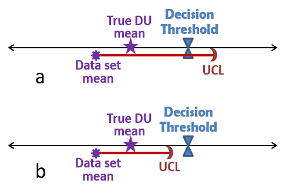
Source: Deana Crumbling, 2020. Used with permission.
Note that the terms “false positive” and “false negative” relate to erroneous rejection or acceptance of the null hypothesis, respectively. Consider a second hypothesis test with the following null and alternative hypotheses for the DU mean:
H0: µ ≤ L, H1: µ > L
For this second hypothesis test, a false positive (incorrectly rejecting H0) would occur if the null hypothesis that the DU is clean were erroneously rejected for the alternative hypothesis that the DU is dirty. Contrast this with what constitutes a false positive for the first hypothesis test shown – that is, erroneously concluding a dirty DU is clean.
For the first hypothesis test, the Type II error would be the probability of erroneously concluding a clean DU is dirty. Strictly speaking, the failure to reject H0 is an inconclusive result unless the tolerance for Type II error is met. However, a tolerance for Type II error is not specified for the hypothesis test. For environmental applications, the DU is often conservatively assumed to be dirty when the null hypothesis µ ≥ L is not rejected (e.g., Figure 3-21b).
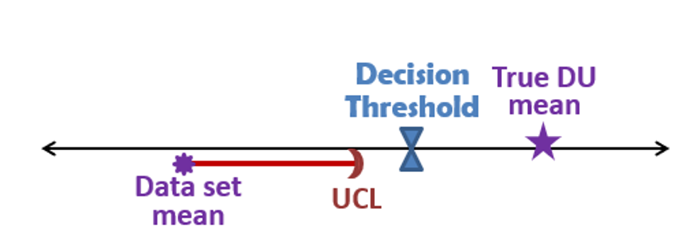
Source: Deana Crumbling, 2020. Used with permission.
It is noted that this approach is conservative from the perspective of human and environmental risk but does not control false negative errors (that is, erroneously concluding a clean DU is dirty). A false negative can occur when the difference between the true DU mean is small, relative to the magnitude of measurement variability. Data variability could be high because of inadequate laboratory sample processing (meaning high subsampling variability). Alternatively, there could have been too few increments to handle the degree of field heterogeneity, producing ISM field replicates with poor precision. The variability (or SD) among the replicates could have increased 95% UCL so the CI overlaps with the threshold (Figure 3-21). Recall that the CI width can be narrowed by collecting more data points, so a solution could be to collect additional DU field replicates (n) or to increase the numbers of increments (k) used to prepare each ISM sample, though the former will likely be more effective than the latter to potentially decrease the 95% UCL to a value below the threshold. Note that if there is very large variability, the original 95% UCL can underestimate the DU mean. Under that circumstance, collecting additional ISM samples could increase the 95% UCL.
3.2.5.2 Underestimation of the DU mean
Under certain circumstances, even ISM may misrepresent the true DU mean, although that is much less likely than with discrete sampling. The cause is the presence of small but significant areas of elevated concentration that are missed by insufficient increment density. This increment density may be too low because the default number of increments was used for a large DU without considering potential areas of elevated concentration, or the areas of elevated concentration are too small to be consistently captured. The existence of areas of elevated concentration increases the overall heterogeneity of the DU, increasing data variability and requiring a higher number of increments to manage.
| Significant areas of elevated concentration denote small areas of increased concentration that have the potential to change a sample concentration from being below the decision threshold to above it if they are captured in their proper spatial proportions by an ISM sample. |
If areas of elevated concentration exist, but their potential presence and configurations are not anticipated in the CSM, the default number of increments could allow a single ISM sample to miss them and underestimate the DU mean. Collecting replicates and calculating 95% UCLs of the DU mean are usually the best strategy for minimizing false positives and underestimating the true DU mean. When sampling DUs with a poorly understood CSM and unknown spatial distributions of contaminants, it is recommended that at least three replicate field samples be collected to estimate the 95% UCL. If all increments of the replicates are evenly placed across the DU, there is a good chance of at least one field sample incorporating at least one area of elevated concentration. The set of ISM samples will likely represent areas of high and low concentrations in the proper proportions for estimating the DU mean and variance. Even one increment picking up a much higher concentration can provide the warning imparted by imprecise field replicate data. If other causes of data variability can be ruled out by QC data, disagreement among field replicates is an indication that more increments may be needed to manage the heterogeneity caused by small areas of elevated concentration.
The following are two examples of areas of elevated concentration causing imprecision among DU replicates of real projects. One of the lessons from these projects is that when heterogeneity is known or suspected to be high, a DU decision based on simple comparison of a single DU field sample to a decision threshold increases the probability of decision error.
| Field Replicate (ppb) | #1 | #2 | #3 |
| DU-A | 380 | 1100 | 1400 |
| DU-B | 460 | 490 | 230 |
The first example is a property adjacent to a landfill that is contaminated with PAHs. The risk driver is BaP, and as shown in the table below, the variability between field replicates DU-A and DU-B is high. This may be due to buried materials that leach BaP into the soil or that weather to shed particles of nearly pure PAHs (such as chunks of old asphalt). Despite 50 increments per field sample for DUs less than 1/10th acre, and with rigorous sample processing that includes milling, the three replicate BaP results can sometimes resemble the two sets below. Note that the BaP cleanup level = 466 ppb (Crumbling 2019).
The other example comes from the Hawaii PCB study (HDOH, 2015). Figure 3-23 shows a 6,000 ft2 (~1/7th acre) area that was known to be contaminated with PCBs (from spilled transformer fluid). This DU was sampled with three field replicates and 60 increments per field sample, with the three replicate PCB results coming in at 19, 24, and 270 ppm (the applicable AL was 50 ppm). The samples were reanalyzed to confirm the accuracy of the results. This level of disagreement is a clear sign of extreme heterogeneity, most likely manifested as small areas of elevated concentration within the DU.
3.2.6 95% UCLs as applied in ISM designs
A question unique to ISM is whether one DU-ISM sample is sufficient (and thus a 95% UCL is not needed) because the ISM sample itself is an estimate of the DU mean. This is a complex topic, so the answer depends on the study question. If the question involves risk-based decision-making, then a 95% UCL may be needed.
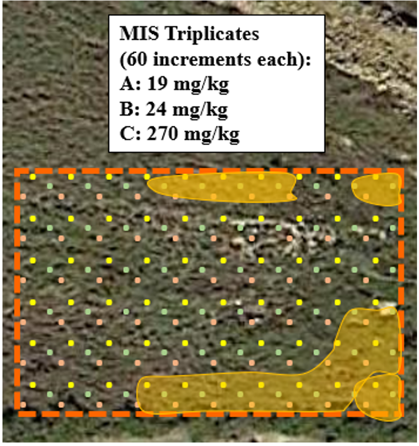
Source: Developed by Deana Crumbling from data by HDOH, 2015. Used with permission.
| Increasing the number of increments, the mass of each increment, or both will increase the likelihood of accurately estimating the true DU mean. |
As was previously shown, it is important to remember that any individual ISM field sample can be significantly larger or smaller than the true DU mean, and it is very unlikely that any result will match the true mean. An incorrect conclusion becomes more likely when the DU is more heterogeneous than expected. At the start of site sampling, at least three independent field replicates are needed to assess variability. If the heterogeneity of the site cannot be assessed before ISM sampling, the number of replicates (or increments) needed may be underestimated. If the underlying population is very heterogeneous, the replicates can have very different estimates of the mean, and the 95% UCL may be elevated. To avoid this, heterogeneity should be assessed whenever possible. After heterogeneity is understood, the sampling design can be optimized. The variability in the DU sample mean depends on the sampling design and can be reduced by increasing the sample support or the number of increments (Figure 3-17). Some sites contain hundreds or thousands of DUs, and 95% UCLs for every DU might not be needed to maintain protectiveness and decision confidence. A statistically sound design for such a strategy is more complicated than basic ISM design: it depends heavily on a mature CSM, an experienced ISM practitioner, and continual evaluation of QC measures.
3.2.6.1 Do not default to “maximum sample concentration”
For the estimation of EPCs using discrete samples, it is a common practice to use the sample maximum (the maximum detected concentration) for the EPC for the EU (that is, the DU) when the 95% UCL of the EU mean is greater than the sample maximum. However, this approach is less likely to provide the desired coverage of the EU mean than the 95% UCL of the mean in most ISM sampling designs. Table 3-4 illustrates the relationship between the ratio of the 95% UCL/maximum for the condition when the underlying distribution of increments is lognormal with CV ranging from 0.1 to 3.
Table 3-5. Probability of the 95% UCL exceeding the maximum concentration.
Source: ITRC ISM Update Team, 2020.
| Replicates (r) | P (95% UCL>max) for Student’s-t | P (95% UCL/max) for Chebyshev |
| 3 | 1.00 | 1.00 |
| 4 | 0.33 | 1.00 |
| 5 | 0.04 | 1.00 |
| 6 | 0.01 | 0.60 |
| 7 | 0 | 0.37 |
| 8 | 0 | 0.18 |
When r = 3, the 95% UCL of the mean will always be larger than the sample maximum. For Student’s-t 95% UCL, the probability is 33% or less for r > 3, whereas for Chebyshev 95% UCL, r > 5 is needed for the maximum replicate result to be lower than the 95% UCL for some sampling events. For r = 3, the ratio of the Chebyshev 95% UCL to the sample maximum is typically less than 1.5.
3.2.6.2 Extrapolating 95% UCLs among CSM-equivalent DUs
Predicting 95% UCLs for single DUs is a strategy that some ISM practitioners are adopting to obtain the uncertainty management benefits of 95% UCLs while avoiding the time and cost of collecting three replicate ISM samples from every DU. However, this strategy should only be applied with CSM-equivalent DUs and is most useful when one or more factors apply:
- There are many (perhaps hundreds) of CSM-equivalent DUs (DUs for which the mechanism of contamination is expected to be similar).
- Multiple rounds of sampling over months or years will be needed to complete sampling of all site DUs.
- There is one contaminant acting as the primary risk driver, and a numerical cleanup criterion has been established.
- More than 30 increments are needed per DU to manage high short-range heterogeneity.
- Increment collection involves the subsurface and more than one depth interval.
- Increment collection is difficult, and refusal is common.
However, replicates should not be collected solely on a frequency basis (such as when three replicates are collected for 10% of the DUs) or a on a per batch basis similar to the manner in which QC samples such as laboratory control samples and matrix spikes (MS) are processed for laboratory analyses. The success of extrapolation methods usually relies on the ability to statistically model the variance or SD for the DUs for which replicates were not collected – for example, the CSM suggests contamination was released in a similar fashion over a larger number of DUs, so it may be desirable to collected replicates for a subset of the DUs. This may be done either in a separate pilot study before the field work begins or at the start of the field program. A statistical test that compares variances (such as an F-test or Levene’s test) may be subsequently used to determine whether the differences in variances of the DUs from which the replicates were collected are statistically significant. If the differences in variances (s) are not significantly significant (95% UCL), the variances can be pooled. The square root of the pooled variance may subsequently be used to calculate s for the DUs for which only one ISM sample was collected. For example, if replicates are collected from m different DUs, Chebyshev UCLs for DUs for which only one replicate was collected may be calculated using the following equation:
![]()
Note that this equation follows from Eq. (3-2) as n = 1 for a DU for which only one ISM sample is collected, and spooled is a pooled SD determined from the variances of the m DUs:
When an equal number of replicates are collected from each DU, the SD formula is simply the square root of the mean variance:
3.2.7 Statistical independence in ISM
A common assumption of many statistical methods is that of independent observations – in other words, the measured value of an SU should not be affected by the value of any other SU. Consider the example of height in individuals. Using the height of two identical twins as two discrete samples and treating them as independent would be inadvisable because the two values are likely to be similar and represent redundant information. The heights are correlated in that they are related, and using correlated values undermines the reliability of statistical analyses.
In environmental data, the assumption of independence may be violated if a DU is stratified into multiple SUs, and there is a spatial trend over the scale of the SUs. If there are multiple SUs that follow a large-scale spatial trend, SUs that are near one another would be potentially correlated and would not be statistically independent. Spatial trends should be taken into consideration during the process of DU delineation to ensure that SUs are independent. If a spatial trend exists within a DU, depending on the size of that DU, the nature of the trend, and the scale of the SUs, a biased estimate of the DU mean can be obtained. However, small-scale spatial trends within an SU do not violate assumptions of independence with ISM data because of the composite nature of ISM (see Section 6.2.2).
In addition to the sampling process, care must be taken during handling procedures to avoid violating the assumption of independence. Suppose a volume of soil representing a single ISM result is not homogenous, and a laboratory subsample is prepared by simply sampling small volumes of soil from only the top portion of the ISM sample. Subsamples prepared in this manner may be more similar than subsamples prepared by collecting soil randomly from different portions of the ISM sample, but the subsample is unlikely to represent the concentration of the entire field sample. For that reason, ISM sample processing involves mixing either by disaggregation and sieving or disaggregation and milling. A one- or two-dimensional (1D or 2D) Japanese slabcake technique with incremental subsampling is then used (see Section 5.3.5).
Staff new to ISM sometimes ask whether field replicates can be collected by splitting a single ISM sample three ways, but this is never recommended because the result actually measures the precision of the splitting process rather than providing three independent estimates of the DU mean.
3.2.8 Application of specialized SUs in ISM projects
The following examples illustrate situations where defined volumes of soil (SUs) are sampled for the purpose of gathering information (such as to refine the CSM) but not to make a decision on the SUs per se. For environmental projects that use ISM, note that such activities are typically conducted to ultimately estimate the DU mean or make a decision about it (say, for a future phase of the project). Please refer to Section 2.
3.2.8.1 Statistical SUs to determine the mean of very large DUs
SUs can be used to statistically determine the mean and 95% UCL for a DU so large that it cannot be sampled as a single unit, provided that the CSM supports relatively homogeneous contaminant concentrations across the entire large DU. In brief, (1) the large DU is completely divided into many equally-sized, spatially contiguous SUs; (2) a random sample of at least 10 SUs is selected from the DU for sampling by ISM; and (3) the SU data are used to calculate the mean and 95% UCL for the DU in the same way as discrete data would be used in ProUCL as described below.
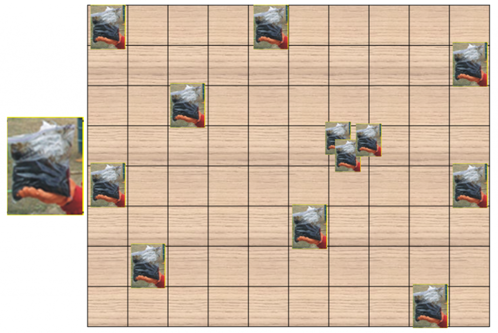
Source: Deana Crumbling, 2020. Used with permission.
As an example, a risk assessor determines that the EU for a farm worker plowing a potentially contaminated field is the acreage of land that can be worked in a day, say, 80 acres. The 80-acre DU is divided into 80 1-acre SUs, and the DU (population) is defined to consist of a set of 80 SUs. Ten of the 80 SUs are randomly selected for ISM sampling (Figure 3-24). Each ISM sample is prepared by randomly collecting 30 increments from the SU. This random selection of both SUs within the DU and increments within each SU helps ensure that a representative statistical sample will be collected.
It may be desirable to collect three replicate 30-increment ISM sampled from one of the 10 SUs for QC purposes – that is, to ensure 30 laboratory subsamples. Three replicate laboratory subsamples are evaluated to ensure that laboratory sample processing and subsampling procedures can control within-sample heterogeneity. Only one 30-increment ISM sample per SU is collected from the nine remaining SUs.
However, only one result from the SU from which three replicates were collected is included in the dataset used to estimate the DU mean because this requires independent data. The three SU replicates are not necessary statistically independent for that purpose (see Section 3.2.6.7) but are potentially related to each other in a way that the other SU data points are not.
DU summary statistics are calculated from the 10 independent SU data points. Because these data points are from different parts of the DU, those data will not necessarily be normally distributed. However, given a sample size of 10, statistical software such as ProUCL can be used to determine whether the results fit a theoretical PD (that is, a normal, lognormal, or gamma distribution) and calculate the 95% UCL of the DU mean. Because CI width (or 95% UCL magnitude) is partly determined by sample size, a determination of compliance (95% UCL ≤ threshold) may be sensitive to the choice of number of SUs.
3.2.8.2 Statistical SUs to make not-to-exceed determinations for very large DUs
As in the example in Section 3.2.8.1, the DU is too large to be sampled as an entire unit. However, instead of determining whether the DU mean exceeds a decision threshold, the goal is to determine whether a proportion of the DU exceeds a threshold. This decision scenario can occur within the context of certain RCRA situations, such as land disposal restrictions. This statistical strategy can be useful in other applications as well.
The strategy is explained in the RCRA’s waste sampling guidance in Section 3.4.2, “Using a Proportion or Percentile to Determine Whether a Waste or Media Meets an Applicable Standard” (USEPA 2002g). Consider the scenario in which the waste material or media at the site (whose boundaries define the spatial extent of a DU) are comprised of a population of unique SUs, each of a defined size, shape, and orientation. Since it is not possible to know the status of all portions of a waste site, we can collect a representative sample and use statistics to support inferences regarding the characteristics of the population. The relevant statistical methods involve calculations of the CI of a proportion (or percentage) of the waste (or DU) that complies with the standard (USEPA 2002g).
The document describes two statistical strategies that could be used, but only the simple exceedance rule method will be discussed here. It is simple because the outcome is either pass or fail, and statistical tables can be used instead of equations. The method is not constrained to a particular PD of concentrations – nonparametric methods are available to achieve acceptable decision error rates. The method is also reliable even in cases of highly censored data (such as a large proportion of the sample results being qualified as non-detects) (USEPA 2002g).
For this strategy to provide an accurate estimate of the mean concentration, the DU must have a relatively homogenous distribution of contaminants. The strategy consists of the following steps: (1) completely divide a large DU into many (more than 100) SUs of equal size; (2) select a subset of n SUs at random; and (3) collect a random sample of increments from each of the n SUs. Refer to Table G-3a in the RCRA guidance (USEPA 2002g)and the equation below to determine the number of SUs (n) that need to be sampled to demonstrate with (1 – α)100% confidence that at least some desired proportion p of the DU is acceptably clean.
For example, based on nonparametric statistics, there is 95% confidence that at least 95% of the DU population is less than the threshold if 59 SUs are sampled and the results reported from all of them are less than the decision threshold. A statistician would describe the maximum reported concentration (from the set of 59 sampled SUs) as a nonparametric 95/95 UTL. By convention, the first of the two values convey the percentile, or coverage (the required proportion of the DU that must be clean), and the second value conveys the magnitude of the upper confidence limit for the percentile. Therefore, a 95/95 UTL is a 95% UCL for a 95th percentile, a 95/90 UTL is a 90% UCL for the 95th percentile, and so on. In general, the number of SUs that must be sampled n to demonstrate at least a proportion p of the DU is clean with (1 – α)100% confidence when the maximum value is less than the standard can be estimated from this equation:
If one or more SU results exceed the standard, we would conclude that the entire DU is not in compliance. If exactly one SU result exceeds the standard, one option may be to continue sampling more SUs (selected at random), effectively to increase the proportion of clean SUs (to approach p). The total sample size (n SUs) required to achieve this result can be calculated explicitly. In general, if one result exceeds the standard, to demonstrate at least a proportion p of the DU is clean with (1 – α)100% confidence, the second largest value reported must be less than the standard, where n is the smallest positive integer that satisfies the inequality:
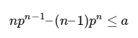
Rather than dividing a large DU into multiple SUs, the same strategy can be used to divide a large study area or property into multiple equal-sized DUs that are randomly sampled using ISM. As an example, a 70-acre former agricultural field is to be developed into ¼-acre residential lots. A review of historical operations suggests the distribution of pesticides is relatively homogeneous across the site, but there is concern that the top 6 in of any single ¼-acre lot could exceed regulatory standards for pesticides. The 70-acre area is divided into 280 ¼-acre residential lot DUs, 59 of which are randomly selected for sampling using ISM samples of 30 increments. Therefore, each SU in this scenario is also a small-area DU. If a 95% UCL is required, either a percentage or all of the ¼-acre DUs would be sampled in three replicates in order to provide an estimate of the variance in the mean concentration.
If none of 59 sampled ¼-acre lots exceed the standard, there is 95% confidence that at least 95% of each ¼-acre lot (sampled and unsampled) in the study area complies with the standard.
The concept of the area sampled within a large DU is very important for risk assessment and risk-based decision-making. When designing a sampling plan to characterize a portion of a large DU and account for potential decision errors from extrapolation, it is helpful to recognize three key factors that can influence the extrapolation uncertainty and likelihood of making a decision error: (1) the variance of the increments (CV of the underlying distribution); (2) the percentage of the large DU area sampled; and (3) the likely magnitude of the average 95% UCL (across all sampled subarea DUs) relative to a compliance level (that is, the ratio of average 95% UCL divided by compliance level). The situation that results in the highest error rates is when the CV is relatively high and the ratio of the average 95% UCL to the compliance level is between 0.1 and 0.4. Ratios lower than this range are extremely unlikely to yield a false negative in which we conclude from the pilot study that unsampled areas of the site are clean when in fact they are not. Likewise, as the average 95% UCL approaches the compliance level (meaning the ratio approaches 1), it is also very unlikely that all the sampled areas will have 95% UCLs that are less than the compliance level (when in fact one or more mean concentrations truly exceed the compliance level). Results of simulation studies that provide error rates for a range of site conditions (CVs), sampling plans (percentage of areas, number of increments and replicates), and 95% UCL calculation methods (Student’s-t and Chebyshev) are available in the White Paper by Goodrum and Mendelsohn (Goodrum and Mendelsohn 2018).
3.2.8.3 SUs to collect spatial information to guide cleanup
A key assumption when defining a DU is that concentration differences within DU boundaries are not important to know – rather, the mean concentration (as estimated conservatively by the 95% UCL) is what matters. While this is true for the primary purpose of the DU, follow-on decisions could arise if the DU concentration exceeds the threshold, and cleanup action is required.
Cleanup must target the contaminated soil, which may or may not exhibit a well-defined spatial distribution. If the bulk of contamination is located in only a portion of the DU, there are many advantages to removing only that portion as opposed to the entire DU. Knowledge of contaminant locations can be ascertained by using SUs designed for that purpose. The DU may be split into several SUs based on professional judgment of where localized contamination is likely present. The DQOs and study questions of the project and soil disposal options can also indicate whether the SU data need to be collected using quantitative ISM samples (30+ increments) or whether composites of only several increments each are acceptable. If the DU mean is near the AL, semi-quantitative data from composites of 5 to 10 increments may not be sufficient to establish where cleanup is needed if risk-based cleanup goals are employed. Because concentrations are near risk-based cleanup goals, a higher degree of precision is needed, and a quantitative approach is recommended.
If other information indicates that cleanup of a DU will likely be needed and returning for follow-up sample collection is undesirable, SUs can be defined at the same time as the initial DU sampling. SU composites can be collected at the same time and held for analysis only if required.
3.3 Planning for the Use of ISM Data
Data collection and evaluation is an iterative process, beginning with the CSM’s development, project planning, analysis, data quality evaluation, CSM revisions, planning of confirmation sampling, and so on. Systematic planning for sampling and analysis is used to support the collection of data whose quality can be robustly evaluated to be sufficient for the intended use of the data. The DQO process introduced in Section 3.1 is a common method for systematic project planning. This section will discuss steps 5 and 6 of the DQO process as it pertains to ISM project planning. Section 3.2 provides an introduction to the statistical concepts discussed in this section.
3.3.1 Decision Rules and Uncertainty
DQO step 5 involves developing an analytic approach prior to receiving the data that will guide analysis of the study results and then drawing conclusions from those data. In this step, the site team specifies what population parameter is most appropriate for making decisions or estimates. It is important to plan for the analysis of the data before they have even been collected. Considerations such as what parameters will be estimated, how uncertainty will be evaluated, and what statistical analyses will be conducted are important to project planning because they may affect aspects of the sample design, such as the appropriate number of samples or number of increments.
ISM samples are estimates of the mean concentration within the DU, and therefore this type of sampling is useful when the average concentration in a particular area is of interest. If the data to be collected will be compared to a threshold or another comparison will be done for the purpose of making a decision, the site team should also specify what level and decision rule they will use in making their decision – for example, whether a 95% UCL will be compared to a screening level or whether a single ISM sample will be used. If the data are being collected to estimate a site parameter, the estimation method should be specified. Moreover, defining the parameter of interest and the decision rule and threshold or the degree of acceptable uncertainty at this point in the sample planning process ensures that the data evaluation will be based on the quality of the sampling methods and the intended use of the data. Once the parameter of interest is identified, step 5 is typically stated in an if-then format to explicitly state the decision rule. If a 95% UCL is compared to a screening level, the statement may appear as, “If the 95% UCL exceeds the AL of X, then take remedial action, else leave the area intact.” In each case, step 5 should explicitly state what remedial action will be taken.
Whereas DQO step 5 considers what the parameter of interest is for the DU and how the data will be used to estimate that parameter, DQO step 6 considers the impact of error and uncertainty on how the data will be interpreted and what level of uncertainty will be considered acceptable. For decision problems, step 5 typically presents decision criteria in the form of if-then statements, but step 6 is essentially a mathematical expression of step 5 that defines the statistical methodology to be used to make a decision selected from a set of mutually exclusive alternates, conclusions, or outcomes. Decision-making problems represent a considerably different type of intended use of the data compared to estimation and other types of problems. The approach to handling and controlling for error and uncertainty associated with the collected data also differs considerably between these two types of problems. As a result, once step 5 of the DQO process is completed, one of two processes is taken in step 6, based upon the intended use of the data: (1) specify performance metrics and acceptable limits of uncertainty (estimation problem) or (2) specify probability limits for false rejection and false acceptance decisions errors (decision problem). Section 3.2 provides an introduction to these statistical concepts. In the example of comparing a UCL to an AL, step 6 would involve defining the confidence of the UCL to limit the acceptable decision error (such as 95%) and setting performance criteria, which in this case, is the target width for the CI.
In the application of ISM samples to a decision problem, one example of a decision rule is comparing a 95% UCL to a threshold to make a decision, where the threshold could be a screening, action, or cleanup level. Confidence limits, which are estimates of the lowest and highest value the true mean might have based on the data collected at a specified confidence level, are important measures for comparisons to the threshold. In particular, where the 95% UCL is below the threshold, the site team has a high confidence in that determination. Similarly, confidence limits may also be important in defining acceptable limits on uncertainty for estimation problems. For estimation purposes, a maximum width of the confidence limit may be specified, typically defined as the distance between the sample mean and the 95% UCL. As discussed in Section 3.2, calculating the CI requires that each DU have three replicate field samples. An exception to this is the unique case of a site with many DUs where the CSM and a statistical evaluation (such as one that uses pilot data) indicates that the heterogeneity of the DUs should be similar. In this case, if sufficient evidence is available to establish the similarity across DUs, the CV of the similar DU could be applied to those missing replicates.
DQO steps 5 and 6 are critical considerations for developing a sampling plan (DQO step 7) and for evaluating the data collected (see Section 6 for further discussion of data evaluation). Defining the parameter of interest and setting acceptable uncertainty or decision error limits during the sample planning provide a clear understanding of how the data will be evaluated and ensure a study design that is likely to achieve the required data quality. The sections below discuss how these steps are applied when using ISM for risk assessment and site characterization (estimation problems) and for comparisons to screening, action, or cleanup levels (decision problems).
3.3.2 Use in risk assessment and site characterization
Two of the most common applications of ISM are site characterization and risk assessment. During this part of the planning process, considerations for each application are essentially the same, the principle difference being in the delineation of DUs (see Section 3.1). For the purposes of site characterization, delineation of DUs should be based on the CSM. If a goal of sampling is to determine if there are spatial patterns of contamination, the DUs should be delineated such that the relationships are not obscured by the composite nature of ISM (see the example in Section 2.5.3). In risk assessment, DUs are typically delineated according to exposure, with the ISM result being representative of the average concentration across the EU (that is, the EPC, see Section 8). The simplest application of ISM to risk assessment occurs when DUs are defined by size and area assumptions of risk – in other words, the DU and the EU are one and the same. These are called exposure area DUs. Due to the inevitable uncertainty in estimates of the mean, regulatory agencies often require a 95% UCL to represent an EPC or to assess compliance with decision criteria (see Section 8).
A variety of different designs are possible for the layout of SUs with regard to their relationship to DUs or EUs (see Figure 1-1). Most commonly, the EPC is calculated using Student’s-t or Chebyshev 95% UCL formulas (see Section 3.2.4.2) across field replicates from a single DU. A second possible design is a large DU that is split into multiple SUs (see Section 3.2.8.2). In this case, the ISM results can be used in the same way to compute a 95% UCL if there is a single ISM sample for each SU, assuming that each SU is equally representative of the DU. This assumption could be violated if, for example, the SUs have different areas or exposure time differs between the SUs.
If there are two or more samples in each SU, a weighted mean could be calculated without having to assume equal representativeness (see the example in Section 6.2.2). However, if multiple replicates are available for one or more SUs, but only a single ISM result is available for other SUs, the method of computing a 95% UCL becomes more complicated because there is no measure of uncertainty available for the SUs with a single result. The results cannot be simply pooled together because the replicates from the same SU will be similar to one another (see Section 6.3.1). In this scenario, three different statistical approaches are possible:
- If there is sufficient evidence to suggest the SUs are similar, the first approach would be to apply the CV from the SUs with multiple replicates to the SUs with a single result (see Section 3.3.1).
- The second approach, which doesn’t require the assumption of similar SUs, would be to randomly select a single ISM result from the SUs for which there are multiples and compute a 95% UCL using one result from each SU. If this approach is used, it is important that the selection of which results are used is truly random. The disadvantage of this approach is that there is a loss of information because some samples will be discarded. The selection and subsequent 95% UCL calculation could be repeated many times to obtain information on how the sample selection process ultimately affects the 95% UCL calculation.
- The third approach is to compute the average for each SU and use each average to calculate a 95% UCL for the larger area. This approach has the advantage that all the data will be utilized, and the 95% UCL will be the same each time it is calculated for the same dataset.
3.3.2.1 QA/QC criteria
Particularly if data will be used for risk assessment, the data should be evaluated to ensure adequate quality. The purpose of any QC activity is to determine whether procedures or methods are working as intended. If any data fail QC criteria, the proper action is to determine the root cause, prevent recurrence, and determine what data have been affected by the failure. Most environmental practitioners are familiar with the concept of QC only in the context of the analytical laboratory, but it is critical for field sampling as well (USEPA 2006b). In general, sampling error is much larger than measurement error and consequently needs a larger proportion of resources to control (USEPA 2006a). As early as 1989, studies showed that sample-related variability contributed most of the total data imprecision (USEPA 1992c). “It has been estimated that up to 90% of all environmental measurement variability can be attributed to the sampling process” (Homsher et al. 1991).
Laboratory-related QC criteria address analyte loss and cross-contamination during laboratory processing, as well as the representativeness (or homogeneity) of laboratory subsamples (see Section 5). Sample-related QC checks evaluate how well each aspect of the sampling design is controlling measurement variability. QC problems signal that the data generation process needs to be improved. Failed QC indicates a problem that potentially affects all samples undergoing the same procedure, not just the ones subjected to the QC check. It is necessary to specify performance criteria prior to data collection, as part of the sample plan or WP. Performance criteria will vary from project to project.
The following procedures measure data variability due to soil heterogeneity at different spatial scales:
- Field duplicates are helpful in ISM to quantify precision of samples from the same SU. For discrete data, this is analogous to co-located samples (a set of two separate samples taken a few inches apart so that their results should be nearly the same). This practice is now infrequently used for discrete sampling because the results rarely agree, and no USEPA guidance makes clear what to do when they do not. Yet USEPA’s Superfund guidance retains a requirement for co-located samples if soil data are to be considered definitive (USEPA 2006b).
- Laboratory duplicates are two subsamples taken from the same field sample for separate analyses. This is another QC practice that is intended to, but frequently does not, produce similar results, especially if heterogeneity is high. When the degree of difference exceeds some limit, guidance says to flag all data in that same batch as “estimated.”
- As part of regulatory oversight, a field sample might be split between the responsible party and regulator field staff for two independent laboratory analyses. Split samples are ostensibly used to ensure the integrity of the implementer’s data, with the procedure resting on the assumption that the splits will have similar concentrations. However, this assumption may not be met, and it is not always clear what should be done if not.
Whatever procedures will be used should be specified during the project planning stages, as well as what measures will be computed, what will indicate an acceptable level of quality, and what action will be taken in the event that quality is not achieved.
Similar measures are used to quantify precision for each of the above procedures. The term precision is different from the term accuracy. Precision describes the reproducibility of the overall sampling method, whereas the accuracy of the data with respect to the true mean concentration of the contaminant in the DU area and volume of soil can only be known by extracting the chemical from the entire volume of soil and measuring the mass. The true error in the data therefore cannot be determined as part of the sampling design. The potential for significant error in environmental decisions can, however, be assessed based on a review of the collection, processing, and analysis of samples, as well as the precision of replicate sample datasets.
RSD is a measure of the precision in replicate samples (typically three replicates) defined as a percentage. It is calculated as the ratio of the SD to the mean, multiplied by 100. Similarly, CV is simply the ratio of the SD to the mean. The RSD can be calculated from either field or laboratory replicates (at least three) to estimate total measurement precision or the laboratory component of variability, respectively. For example, a low RSD from three field replicates indicates good precision in the sampling method used, which may indicate data for similar DUs collected under the same design have good reproducibility and reliability. However, the determination of what is “good” is highly subjective and may vary from project to project, so this should be specified during project planning. For specific examples of CVs that may indicate 95% UCL estimation reliability, refer to Table 3-3 in Section 3.2.4.2. Note that high RSDs can become unavoidable as contaminant concentrations approach the laboratory method reporting and detection limits.
Similarly, the relative percent difference (RPD) is the percent difference between two sample results that are expected to have the same true concentration. The RPD is calculated for field or laboratory duplicate results to evaluate the precision of the sampling design and measurement system. In concept, the RPD and RSD are similar metrics, but RPD is used for duplicates whereas RSD can be used for upward of three samples. Although a 30% RPD or RSD has emerged as a typical standard, in reality, the RPD/RSD depends on the analytical methodology as well as the analyte. The target RPD/RSD should depend on the project objectives and be within the capabilities of the measurement system.
Completeness is a sampling design term defined as the minimum number of sample results (data points) needed for each analyte and DU to meet each data use objective, relative to the number of usable results that are available or planned. Completeness criteria should be specified in the WP or QAPP. Recovery is a measure of the agreement of an experimental determination and the true value of the parameter, and is used to identify bias in a given measurement system. Standards for recovery criteria depend on the analytical methodology and are available in the U.S. Department of Defense’s Quality Systems Manual (QSM) Appendix C (DOD/DOE 2018) (see also USEPA SW-846 (USEPA 2007)). These standards do not account for ISM sample preparation procedures (see Section 5), but they could be used as a loose guide for determining recovery criteria.
3.3.3 Comparison to endpoints
Another common application of ISM is in a decision problem, as described in USEPA’s DQO guidance, which involves comparing sample results (typically, a 95% UCL) to a numerical criterion of some sort. Cleanup levels, also called remedial goals, are an example of such a criterion. Cleanup levels may be defined in a variety of ways, including regulatory standards, or based on risk assessment calculations under applicable guidance. The specific set of criteria will vary from project to project, but considerations for applying ISM data for these comparisons are consistent across all types of numerical criteria.
Many cleanup levels are developed based on a set of assumptions about the exposure to humans and ecosystems, including the size and location of EUs. When sampling to compare site concentrations to a cleanup level, the area of the EU or DU should be compatible with the exposure assumptions used to develop the cleanup level. If the EU is much larger than the assumed exposure area used to develop the cleanup level, receptors may be exposed unequally to subareas of the EU, and unacceptable levels of contamination may be left unaddressed. For example, comparison of ISM results for a 2-acre DU to a risk-based cleanup level might be appropriate for cleanup levels pertaining to an ecological or recreational endpoint, but might be considered inappropriate for a residential endpoint. These considerations should be addressed in the planning process. Comparisons of ISM results to cleanup levels should also appropriately account for the possibility of a decision error (for more detailed discussion, refer to Section 3.2). Practitioners must consider what probability of each type of error is acceptable. Generally, practitioners would rather make the mistake of remediating a site that is already clean than make the mistake of not remediating a site that is contaminated.
While a common decision rule is comparing the cleanup level to a 95% UCL, the choice of decision rule may vary from project to project (see Section 6.2.1 and USEPA 1989). In the example of calculating a 95% UCL and comparing this value to a cleanup level, the probability of concluding that the mean is less than the cleanup level when it is actually greater is 5%. Therefore, this decision rule can be applied if the acceptable error rate for this decision is deemed to be 5%. Specifics for computing 95% UCLs for risk assessment under various sampling designs (see Section 3.3.2 and Section 8.3.3.1) are also applicable for comparisons to any cleanup level.
3.3.3.1 Considering decision errors and sample sizes
Identification of acceptable rates for each type of error is important information that can be used to determine how much data need to be collected. As acceptable error rates decrease, it is necessary to be more confident that the decision made is the correct one, and more information is needed to make a statistically valid conclusion. This could come in the form of an increased number of increments or additional ISM samples. A power analysis could also be performed to calculate the precise number of samples that would be needed to achieve acceptable error rates.
Increasing the number of increments collected increases confidence that any one ISM result is a good estimate of the mean concentration in the area of interest. Similarly, increasing the number of ISM samples collected increases the confidence that the true mean has been captured in the collection of sample results. Both result in a narrower CI width (see Section 3.2.4.3), therefore, the mass of soil collected ultimately affects the probability of making a decision error in subsequent analyses.
In any decision problem, two types of errors are possible. When a 95% UCL is calculated, the probability of concluding that the site is clean when it is truly contaminated is equal to 0.05 (false compliance, α). The opposite error is concluding that the site is contaminated when it is truly clean (false exceedance). While confidence is one minus the false compliance rate, one minus the false exceedance rate is known as power. Statistically, power is the probability of obtaining a significant result when the result is truly significant. In this case, power refers to the probability of concluding that the site is clean (the 95% UCL is below the AL), given it is truly clean (the true mean is below the AL). For a specified number of ISM samples, lowering the tolerable false compliance error rate will result in decreased power.
In order to inform the number of samples needed for desired error rates, a power analysis could be conducted if information is available on how much variation is expected in the data and how far site concentrations are from the AL. Such analyses must be done a priori. Given known variation in the data, the relationship between power, α, n, and the detectable difference is quantifiable by many publicly available online calculators, as well as the pwr package in R. The detectable difference is the minimum difference that can be detected by statistical analysis with a probability equal to the power. In the case of comparison to a numerical criterion, the detectable difference is the difference between the true site mean and the threshold or cleanup level. Because certain information about the site is needed for a power analysis, it is most useful for sites where a pilot study or characterization of a similar area has already been conducted. The variance of those data could be used as a surrogate in the analysis. The more variation in the data, the greater number of samples required to achieve the desired power at the required significance level. In addition, it is necessary to have a general idea of the concentrations that may exist in the area of interest in order to define the difference the analysis should detect. Typically, this is the difference between the threshold or cleanup level and the true site mean. Since the true site mean is unknown, power could be calculated using multiple values for the detectable difference as well as and power, and a somewhat subjective decision could be made taking into account cost, power, the detectable difference, and the ability to collect additional samples.
An example of a power analysis on a real dataset is given in Table 3-6 for Pb. In this case, data from a similar area were available, so the sample SD of the observations (that is, measurements of environmental samples) from that area was used in the calculations, which assumed that the data were independent and approximately normally distributed (see Section 6.3), and a 95% UCL would be compared to the screening level. The sample mean Pb concentration for the surrogate area was 25% lower than the screening level. The estimated detectable difference between the population mean and the screening level is assumed to be 25%, but sample sizes are also computed for 15% and 35% differences to inform decisions. In this example, a more conservative approach would be to assume the true difference is lower than 25% (say, 15%). For a multi-phased sampling design, it may be more cost-effective to use 25% or even 35% and resample the area in subsequent phases if necessary. Note that power calculations could give sample sizes less than three, but three replicates are still required to compute a 95% UCL.
Table 3-6. Example power analysis results for sample sizes required to detect true differences of 15%, 25%, and 35%.
Source: Hayley Brittingham, Neptune and Company, Inc. Used with permission.
| 15% Difference | |||
| 1% False Compliance ( α= 0.01) |
5% False Compliance ( α= 0.05) |
10% False Compliance ( α= 0.1) |
|
| 30% False Exceedance (power = 0.7) |
11 | 6 | 5 |
| 20% False Exceedance (power = 0.8) |
13 | 8 | 6 |
| 10% False Exceedance (power = 0.9) |
15 | 10 | 8 |
| 25% Difference | |||
| 1% False Compliance ( α = 0.01) |
5% False Compliance ( α = 0.05) |
10% False Compliance ( α = 0.1) |
|
| 30% False Exceedance (power = 0.7) |
6 | 4 | 3 |
| 20% False Exceedance (power = 0.8) |
7 | 4 | 3 |
| 10% False Exceedance (power = 0.9) |
8 | 5 | 4 |
| 35% Difference | |||
| 1% False Compliance ( α = 0.01) |
5% False Compliance ( α = 0.05) |
10% False Compliance ( α = 0.1) |
|
| 30% False Exceedance (power = 0.7) |
5 | 3 | < 3 |
| 20% False Exceedance (power = 0.8) |
5 | 3 | 3 |
| 10% False Exceedance (power = 0.9) |
6 | 4 | 3 |
Another important consideration in estimating sample size is the selected values of false exceedance and false compliance rates. Most commonly, practitioners are satisfied with a 5% probability of false compliance error (α = 0.05) and a 20% probability of false exceedance (power = 0.8). However, it is worth considering deviating from this convention depending on the needs of a particular site. As an example, α = 0.01 might be appropriate for sites with a larger volume of people living close by. If remediation is especially costly, practitioners may decide it is worth collecting additional samples to avoid the risk of remediating a site that is already clean (false exceedance). In the example above, increasing the number of samples from 4 to 5 would decrease the chances of false exceedance from 20% to 10% (assuming a 25% detectable difference and α = 0.05).
The power analysis is only one line of evidence to inform appropriate sample size. For example, in the case of large DUs made up of smaller SUs, a certain level of spatial coverage may be desired to adequately characterize the entire DU (such as 10% of the potential SUs). Qualitative judgments such as the level of skew in the data or a desire for increased confidence or power may also be used as a justification for additional samples or increments. See Section 3.2.8.1 and Section 3.2.8.2 for statistical discussion of large DUs made up of smaller SUs.
3.3.4 Background comparisons
Another common study objective is to compare ISM site data to background concentrations. This comparison requires different statistical methods than those used to compare ISM site data to numerical criterion or cleanup levels. While cleanup levels are known constants, background concentrations are variable, and the true mean and maximum background concentrations are unknown. Comparing site data to background concentrations involves relating two different distributions (site and background) and requires a hypothesis test (such as a two-sample t-test) to determine whether the concentrations are similar (see Section 3.2.5.1). Comparing ISM samples to background concentrations is most straightforward when both site samples and background samples are collected using ISM and with similar sampling characteristics such as the number of increments and the total volume of soil per sample (see Section 3.1.6.2). While statistics exist to compare ISM samples to other types of samples, these methods are complex and require the assistance of a qualified statistician. With any statistical method, predefining acceptable error rates is an important part of the planning process.
It is important to check the assumptions of the chosen test after data collection to ensure that the test is appropriate (see Section 6.3). Some practical tests for comparison of site ISM samples to background ISM samples are discussed in the following sections. For more information on these comparison methods, see the White Paper (Georgian 2020).
3.3.4.1 Comparison of means
For risk-based environmental applications, it is preferable to use hypothesis tests to compare mean site and background concentrations. Two-sample t-tests are commonly used for this comparison because they only require that both distributions are roughly normally distributed, which is generally achieved for ISM samples through physical averaging and the CLT. A two-sample t-test compares the means of the site and background distributions with a prescribed confidence level, such that the null hypothesis is only overturned if there is strong evidence that the site is actually contaminated. Statistical terminology and decision points include error rates, statements of null and alternative hypotheses, and one- and two-sided tests.
Hypothesis testing involves two key concepts regarding the definitions of null and alternative hypotheses. The first concept involves the definition of the null and alternative hypotheses as inequalities. When conducting a background screening analysis, we are most interested in evaluating whether the site mean is greater than the background mean, and whether the difference in means is greater than some prespecified substantial amount S. If so, the null hypothesis is expressed as an inequality, and the term one-sided (or one-tailed) test is used. With one-sided hypothesis tests, the false compliance error rate is often α = 0.05. The second concept involves the direction of the inequality. When doing a one-sided test, we can elect to use either of the following conditions for the null hypothesis H0, and alternative hypothesis HA:
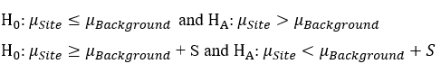
USEPA describes these options as Background Test Form 1 and Background Test Form 2, respectively (USEPA 2002b, 2015). The two approaches can yield different conclusions when the difference between the site mean and background mean approach S. Some regulators prefer Background Test Form 2 because it puts the burden of proof on the data to demonstrate that the site mean is not elevated (USEPA 2002b).
Because it may require more samples than are typically collected via ISM to identify small differences between the site and background means, it may be desirable to consider looking for at least a minimum meaningful difference between the site and the background means, instead of looking for just any discernable level of difference. The hypothesis test can be set up to consider any difference or only to discern at least a particular (ideally meaningful) difference.
If the assumption of normality is not well met for either the site or background data, then a nonparametric test for comparison of medians might be appropriate. Nonparametric tests such as the Wilcoxon-Mann-Whitney test, Sign test, or Permutation test may be used to compare the midpoints (means or medians, depending on the test) of the site and background datasets and achieve error rates even under conditions of non-normality. Note that while nonparametric tests relax the assumption of normality, they do not relax the assumption of equal variance (meaning the test can yield higher than expected error rates if the variances of the site and background distributions are different).
An analysis of variance (ANOVA) test may be used to compare the means of two or more SUs. ANOVA is a parametric test that compares the means of two or more sites to determine whether any of the site means are statistically different from one another. The null hypothesis for the ANOVA test is that all the site means are equal. The alternative hypothesis is that not all the site means are equal (that is, at least two site means are different). If comparing just one site to background, the replicate background samples will be compared to the replicate site samples to determine if they have statistically similar means. A strength of the ANOVA approach is that it is just as possible to compare several sites at once, so one background dataset could be compared to the data from several SUs. Note that an important caveat when evaluating multiple groups is that because the null and alternative hypotheses cannot be defined as inequalities, ANOVA is inherently a two-sided test of differences in means (or medians for nonparametric options). Also, if the null hypothesis is rejected, that would only mean that at least two of the sites differ, and it would not be clear which sites those are without further evaluation. Inclusion of multiple sites simultaneously in an ANOVA may require follow-up by individual comparisons of each site to background to determine which one (or more) site is statistically greater than background.
Power analysis. A power analysis may be conducted using the acceptable error rates in concert with information on the variance and the minimum difference the analysis should detect. Most online calculators and commercial software for statistical analysis can calculate the power. Such an analysis may also be conducted in the context of a background test, but the interpretation of the false exceedance error and corresponding power may differ from that of a one-sample hypothesis test (such as comparison to a threshold) depending on how the null hypothesis for comparison to background is defined. Also, the decision to apply a Background Form 1 or Background Form 2 approach can affect the statistical power, given the prescribed sample sizes and S. In the case of Form 2, the null hypothesis is that the site mean is greater than the background mean by at least S. Therefore, the following definitions of error and power apply:
- False compliance error (α) is the false positive condition – the probability of (falsely) concluding that the site mean is not contaminated above background by S (reject H0), when it truly is elevated by more than S.
- False exceedance (β) is the false negative condition – the probability of (falsely) concluding that the site mean is greater than or equal to the background mean by S (do not reject H0), when it is not truly elevated.
- The corresponding power (1 – β) is the probability of not falsely concluding that the site mean is greater than or equal to the background mean by S.
3.3.4.2 Comparison of the upper tails
In addition to comparison of the mean concentrations, it could be useful to compare site concentrations to an estimate of the upper tail of the distribution of background concentrations. The Quantile test compares the upper percentile (such as the 95th percentile) of both distributions (Gilbert 1987). If the upper percentiles of the site concentrations substantially exceed the corresponding upper percentile of background, it could suggest that small pockets of elevated concentrations exist on site that may not be consistent with background. Relating a single ISM site sample to a distribution of background concentrations is also possible (such as a 95% upper prediction limit [UPL] or 95/95 UTL). This comparison is useful if the objective is to merely demonstrate that a release above background has occurred. If normality can be assumed, UPLs may be an option for evaluating future ISM site means (USEPA 2009). Some simulation studies with UPLs demonstrated that desired power can be achieved even for small sample sizes and some non-detects in the background ISM dataset (Georgian 2020). However, simulation studies of the statistical performance of 95/95% UTLs clearly illustrate that the UTL lacks statistical power, given the usual sample sizes for ISM investigations, and can lead to much greater decision error rates than expected (Pooler et al. 2018). If achieving a high degree of confidence in conclusions related to background is critical, point-by-point comparisons to UTLs may not meet project objectives. In general, hypothesis testing is preferred over point-by-point approaches. As a supplemental exploratory data analysis step, it is also always useful to compare the sample results qualitatively, noting whether they appear similar, whether the greatest value falls in the background or the site dataset (this can also be quantitatively assessed using the Slippage test (Gilbert 1987)), and noting whether there are a similar percentage of non-detected results.
3.4 Cost-Benefit Analysis
A sampling protocol is often limited by how much funding resources are available to the property owner and/or responsible party. Thus, a sampling plan is often designed based on limited traditional sampling methodologies (that is, discrete and/or composite sampling approaches) to fit into a preexisting budget instead of an unbiased identification of the data required to meet project objectives. The result is often limited data with a high risk for decision errors. As stated in Section 2.2, heterogeneity causes sample analytical results to fluctuate depending on the precise location, particle segregation, cohesiveness, and sample mass. ISM generally yields more precise and unbiased estimates of the mean, and the cost-benefit ratio often favors the ISM investigation because it results in fewer decision errors. Less data variability will likely allow for less uncertainty in decision-making, especially when estimates of the mean are close to an AL.
This section will assist in determining potential costs associated with implementing ISM and reference case studies to help determine the cost-benefit of utilizing ISM for a specific site. Proper planning is a major factor for designing the most cost-effective implementation of ISM (described in Section 3).
3.4.1 Costs and benefits of ISM
A simple and direct cost comparison of ISM to traditional sampling approaches is difficult due to several factors, including analytical costs, availability and quality of screening technologies, sample collection methodologies, and establishment of a clear endpoint to a project.
Keep in mind for the ISM versus discrete sample examples presented that the precision and representativeness of a single set of discrete sample data for estimation of the mean is never known, since replicate sets of discrete samples are not collected for comparison. This can impose significant uncertainty and future liability concerns for projects and is the root cause of many failed investigations and remedial actions. Unfortunately, this type of uncertainty is not easily quantifiable. As a common saying in the environmental industry goes, “How much is a lawsuit going to cost you?”
The following section describes comparative costs and considerations for project-specific evaluations. In general, ISM may have higher planning and sampling preparation costs compared to traditional sampling methods. However, providing a reliable and adequate dataset using ISM offers the potential to limit substantial costs that could otherwise be incurred due to additional sampling needs and/or unnecessary remediation.
3.4.1.1 Financial
Variations in costs between ISM and more traditional sampling methods typically occur during system planning, sampling plan review, field sampling, and laboratory services of a project. These four areas are discussed further below.
Systematic planning. Systematic planning that includes the designation of DUs, sample protocol, and associated decision statements to guide data evaluation, while being a key component of ISM investigations, is not unique to ISM, which requires the upfront consideration of DUs and associated decision statements. Although this should be done prior to any project involving soil sample collection, a more detailed planning process is required for ISM.
Omission of a more detailed planning process using discrete and/or composite sample methodology often results in multiple sample collection events to complete site characterization, followed by the designation of impacted areas using limited site characterization data on which final decision-making is based. This process often leads to the need for additional site investigations to fill data gaps or and/or final decisions based on limited data not necessarily reflective of the actual risks posed by contamination at the site.
Systematic planning costs should be roughly equivalent regardless of the sampling design. Developing DUs, discussing hot spots, including additional staff to participate in planning meetings, and stakeholder agreement may increase front-end costs but can significantly reduce cost and the need for lengthy discussions following completion of the field investigation. The intent of systematic planning is to collect usable data and minimize the need for remobilization to collect additional data or situations where parties disagree on the size of a hot spot. Eliminating both would result in lower overall cost in the project lifecycle.
| UFP-QAPP worksheets are an ideal format to guide teams through systematic planning and ISM design. |
Sampling plan review. A common concern of both regulators and the regulated community is ISM sampling plan review. For regulators not trained in ISM investigation approaches, the sampling plan review can be labor-intensive. For consultants, the time required for regulatory approval of ISM projects from agencies that lack adequate training and guidance documents also increases costs to their clients and at least perceived risk of rejection. In addition, many consultants find it much easier to submit standard sampling plans and assessment/remediation reports to regulators with the goal of a quicker turnaround time for their clients even if they know that this approach will ultimately result in a more drawn out and costly investigation over the life of the project. However, with time, education, and familiarity with the ISM method, the comparative costs for sample plan review will decrease to become comparable with more traditional sampling technologies.
Field sampling. Many factors can affect the cost of ISM field sampling. All costs are highly dependent on the DQOs, and the size and number of DUs has a direct effect on the financial cost of the field effort as well. A demonstration completed by (USACE 2013a) specifically to evaluate ISM costs and performance at three shooting range sites indicated that “ISM can result in a cost savings of 30% to 60% relative to conventional grab sampling methods.” Areas of cost savings in the field include the following:
- A reduced number of samples need to be prepared for laboratory analysis.
- Fewer sample supplies are consumed.
- Decontamination of field equipment is only required between DUs.
- Less time is required to survey as only the corners of the DU need to be identified.
The collection of MIs results in a longer collection time per sample than that for a single discrete sample, but that said, a relatively large number of discrete samples are needed to provide the same data quality as ISM. For the purposes of this chapter, surface sampling was used to compare costs between ISM and traditional methods only. Subsurface ISM sampling may result in higher field costs depending on the sampling method and should be considered on a site-by-site basis.
Laboratory services. As stated above, ISM decreases the number of samples analyzed to characterize a site compared with discrete sampling. For example, a DU will include analysis of three replicate ISM samples, but typically a minimum of 8 to 10 discrete samples are necessary, and as many as 20 discrete samples are commonly recommended by ProUCL guidance for risk assessment purposes, depending on analyte variability. In addition to laboratory analysis, CLP-like data packages and data validation will cost less for ISM projects as there are fewer samples requiring analysis and validation.
| If the overall project costs for ISM are higher than that using discrete methods for a specific project; it is worthwhile to double check if you are adequately meeting your DQOs with traditional methods. |
However, the cost savings for laboratory analysis is not solely based on the total number of samples. For ISM, it is recommended that sample processing (such as drying, sieving, and milling) is handled by the laboratory and not completed in the field. The ISM laboratory sample processing and subsampling options are described in Section 5. The price of ISM processing depends on the specific options selected, the amount of soil, the analytes of concern, and other general concerns (such as the number of samples and turnaround time). Understandably, laboratories charge for ISM sample preparation, and rates are in the range of $65 to $200 per sample, depending on the sample preparation methods required to meet the DQOs. Per sample laboratory costs, including processing, QA/QC, and analysis, can double for a single discrete sample; the savings for ISM is achieved because fewer samples are required to adequately characterize an area.
Laboratory costs will increase proportionally with the number of DUs, but savings are realized by using ISM because more discrete samples are typically required for the same spatial coverage. Further, field labor costs using ISM can be absorbed by the decrease in laboratory costs if remobilization for additional discrete sampling is required, to complete needless remediation, or to address the potential damages and legal expenses of not appropriately assessing the magnitude and limits of contamination.
3.4.1.2 Cost variations
The actual cost differences between the sample methodologies will vary from project to project based on several factors. Some of the more critical factors are the number of discrete samples required to generate a statistically defendable dataset and meet the DQOs and the actual time required to collect such samples. Other lesser factors include the following:
- the size of the property and nature of the release
- individual analyte costs
- the use of field analytical methods for specific contaminants
- the ISM sample processing method (drying, particle size reduction, sieving, subsampling)
- the presence of clay, roots, and very wet soil (likely increases overall field processing time and potentially increases costs)
- increased ISM laboratory charges for difficulties sieving the soil (clay, roots, very wet)
- the potential cost of extra ISM QC samples (that is, batch samples)
- the potential cost of large volume shipping and disposal for ISM soil/sediment projects
The link below provides a simplified comparison of field and laboratory costs for ISM and discrete sampling methods but should not be considered comprehensive. It is an interactive table such that the number of DUs and other applicable parameters can be entered, and a series of general assumptions for a generalized estimate will be provided for both methods. This table is meant to provide an example of costs for different sampling scenarios and should not be used for site-specific project estimating purposes.
ISM versus Discrete Cost Comparison Work Sheet for estimates of ISM verses discrete sampling field and laboratory costs
3.4.1.3 Schedule
As described in Section 3.3, completion of ISM requires additional systematic planning to determine the DQOs, determine the number and location of DUs, and sampling requirements. The additional planning will require additional time in the project schedule, potentially more than other sampling methods – the field schedule is more or less equal. Experience has shown that 30-sample increments in three replicates can be collected in approximately 45 minutes with two people provided the DU is less than a ¼ acre. Collection of 8 to 20 discrete surface samples in the same area would be comparable considering that decontamination would be required in between each sample and each sample would be logged and labeled for submittal to the laboratory. Additional time will be required by the laboratory for ISM sample processing, which should be considered if an expedited turnaround on sample results is required. A delay in project schedule may also occur for the review of planning documents, especially as the industry is understanding proper ISM implementation methods and procedures, which is one of the main goals of this document. These delays can be partially mitigated by increased knowledge, experience, and additional staff. Figure 3-26 provides a graphical representation of generalized project schedule with and without ISM.
Source: ITRC ISM Update Team, 2020.
3.4.1.4 Decision error
Section 3.2 describes the statistical concepts behind ISM and the importance of producing statistically defendable data. Due to the nature of sampling, it is entirely possible to collect discrete samples from the same area twice and come up with contradicting conclusions regarding characterization. Without proper data, it is possible to conclude a site is dirty when it is clean or that a site is clean when it is dirty. This can lead to multiple investigations, project delays, implementation of an inappropriate remedial action, and an increased liability to the property owner, regulatory agency(ies), and project stakeholders. All of these outcomes will increase costs.
| ISM provides much higher confidence in cleanup decisions, which helps ensure effective use of funds toward addressing actual environmental impacts. |
3.4.1.5 Environmental impact
While less tangible than previous factors, there is a potential for inadequate characterization as it pertains to undetermined risks to human health and the environment. As environmental professionals, we understand that there are risks of incomplete assessment with all methods and techniques, and limiting that risk is our primary goal and responsibility. Therefore, employing a technically and statistically defendable method for assessment of soil is the most prudent course of action.
3.4.2 Examples
This next section provides examples that compare the costs and benefits of using ISM to more conventional sampling methods.
3.4.2.1 Site screening
ISM provides significant advantages for site screening, especially if the mode of contaminant dispersion is generally uniform across large areas. Specific examples where ISM has been used include munitions sites or ranges (including small-arms and skeet and trap ranges), former mines, landfills, and sites that were contaminated by surface application of pesticides and/or herbicides, radiation, and/or PCBs. Sites where an overall assessment of potential site risk to known receptors is required here. While this may seem counterintuitive, it is important to recognize that the statistical basis for ISM matches well with the contaminant distribution at these types of sites.
Site screening with ISM is very well suited when little information is known about the site and/or access is limited, when data collection will take place in a single mobilization (brownfield site planned or already developed for residential and/or commercial development), and a full analyte list is required. ISM provides a more complete and reliable dataset, minimizing the potential for remobilization, “step out” sampling, and data gap investigations. The case studies in Appendix A offer various examples of ISM applications on range sites, brownfields redevelopment sites, and sites with historical herbicide and pesticide application. The following examples illustrate the potential cost benefits of using ISM for site screening.
Example 1: small-arms practice range. In this example, a former small-arms practice range requires screening to assess if impacts to soil have occurred that are a risk to human health and the environment. No historical sampling has been performed, but impacts to surface soil are likely due to the accumulation and degradation of bullet fragments during range operation. In this case, the site configuration and prior use can be used to select the SUs for investigation. In Figure 3-27, a total of five SUs were selected based on the CSM identifying the likely areas of impacted soil. SUs are used in this example because the data will be used for site screening and not for decision-making purposes. See Section 3.1 for further discussion on the application of SUs and DUs.
Here, three replicate ISM samples from each SU for a total of 15 samples will be submitted for laboratory analysis. Guidance for small-arms range sites recommend that at least 50 increments are collected for each SU due to the typical size of the SUs, nature of contaminant distribution, and likelihood for contaminant heterogeneity. In this example, 50 increments are selected for the range floor and 30 increments for the firing line, target berm, and two side berms as these areas are significantly smaller and therefore less likely to be impacted by contaminant heterogeneity. (See Section 2.5.2 for a discussion on the selection of the number of increments for a specific SU.) This sampling program will collect soil from 510 locations, including increments for each replicate sample.
Source: ITRC ISM Update Team, 2020.
Source: ITRC ISM Update Team, 2020.
Table 3-7. Number of ISM verses discrete samples at a small-arms practice range.
Source: ITRC ISM Update Team, 2020.
| DU | # of ISM Samples | # of Discrete Samples | |||
| Investigation | Replicates | Increments | Investigation | Duplicates | |
| Firing Line | 1 | 2 | 90 | 10 | 1 |
| Range Floor | 1 | 2 | 150 | 50 | 5 |
| Side Berm 1 | 1 | 2 | 90 | 20 | 2 |
| Side Berm 2 | 1 | 2 | 90 | 20 | 2 |
| Target Berm | 1 | 2 | 90 | 20 | 2 |
| Total | 5 | 10 | 510 | 120 | 12 |
For comparison, a typical and statistically comparable set of discrete samples were also considered, and a total of 120 discrete soil sample locations were selected: 10 locations near the firing line, 20 locations in each side berm, 20 locations in the target berm, and 50 locations for the range floor.
Consistent with ISM, all samples will be analyzed for metals, and the locations at the firing line will be analyzed for metals and explosive residues. All ISM samples will be prepared by drying, sieving, milling, and subsampling by the laboratory. Using the comparison cost calculator presented in Section 3.4.1.1, the field and laboratory costs are estimated as in Table 3-8.
Table 3-8. Cost estimate for field and laboratory costs for ISM verses discrete sampling at small-arms practice range.
Source: ITRC ISM Update Team, 2020.

The financial costs for this field mobilization using ISM are a quarter of the costs for a discrete sampling program. The likelihood of remobilization is unlikely for this site since the area of impact is well-defined to the area of the range. Other benefits of ISM include greater representation of contaminants, more accurate decision-making that will ultimately result in an appropriate determination of risk, and selection of the most appropriate remedial alternative.
3.4.2.2 Remedial investigation and risk assessment
The remedial investigation process defines the nature and extent of environmental impacts and provides data for risk assessment. Because risk assessment is typically interested in characterizing average exposure to human or ecological receptors, ISM is more directly related to risk assessment than discrete sampling. ISM includes an added component of replicate sample data that can be used to assess the precision and reproducibility of the overall sampling method, increasing confidence in decision-making. Confidence in the resulting data is also increased because ISM typically provides greater coverage of a targeted exposure area and incorporates sampling theory requirements for minimum sample mass, as well as strict processing and analysis requirements. Such considerations are not typically incorporated into discrete sample investigations. Also, because ISM provides and higher sampling density and better spatial coverage within the DU, the confidence in the average analyte concentrations is typically higher than for discrete sampling. Case studies have demonstrated that ISM is applicable to evaluate nature and extent as well as human health and ecological risk assessment processes. Additionally, short-term delay to prepare for and execute ISM has reduced the need to remobilize to the field and resulted in a more complete dataset for evaluation of risk and remedial alternatives.
Example 2: soil sampling of a liquid spill. In this example, a chemical in solution or liquid waste is accidentally released to soil from two abandoned drums on a flat terrain (Figures 3-29 and 3-30). The liquid containing the chemical of interest (COI), in this case an SVOC, flows out from the source. It is assumed the concentration of the COI decreases with distance from the point of the spill, as shown in the diagram below. Three concentric circles of concentration, representing high, medium, and low, have been constructed and are assumed to be the SUs, but these SUs are likely to be of different sizes. Ideally, the boundaries of these SUs would represent a transition boundary at the COI soil screening level, which we assume for this example has been previously established. Area 1 represents 0.4 acres, Area 2 is 1.2 acres, and Area 3 is 2.4 acres. SUs are used in this example because the goal of the assessment is to define the lateral extent and not for risk characterization. See Section 3.1 for further discussion on the application of SUs and DUs.
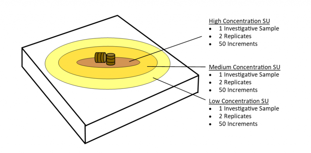
Source: ITRC ISM Update Team, 2020.
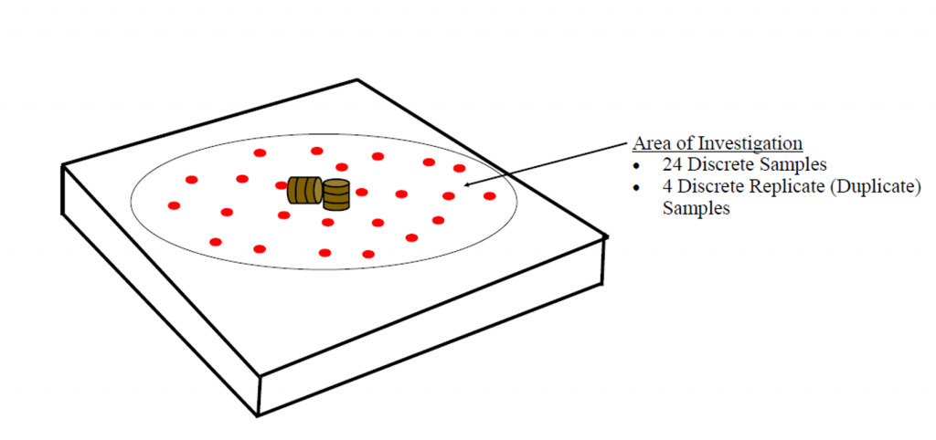
Source: ITRC ISM Update Team, 2020.
For ISM samples (Figure 3-29), 50 increments are considered better because of potential SVOC soil adherence. Assuming three replicate ISM samples, the calculator indicated a cost of $9,600 see Table 3-9). For comparison, a total of eight discrete surface samples were randomly selected for the same area represented as an SU (Figure 3-30). Using the cost comparison work sheet presented in Section 3.4.1.1, the field and laboratory costs are estimated as in Table 3-9.
Table 3-9. Cost estimate for field and laboratory costs for ISM verses discrete sampling for soil sampling of a liquid spill.
Source: ITRC ISM Update Team, 2020.

The costs for ISM in this example are lower than that of discrete sampling. The potential advantage of discrete sampling is that each sample may provide information on the possible boundary for soil above or below the soil screening level, but the method is relying on eight samples to provide an accurate concentration, especially in Area 3 (eight samples for 2.4 acres). ISM sampling will provide a better measurement of the mean for the SU.
3.4.2.3 Remedial action
Following remedial action, ISM can provide greater confidence that target cleanup and risk goals have been met. For example, soil excavation typically requires confirmation samples at the base and sidewalls to the removal of impacted soil. Accordingly, ISM sampling that sets each sidewall and the floor as a DU would reduce the decision error associated with discrete sampling results that mis-characterize the remaining contamination and lower the potential for needless continued costly excavation and soil treatment.
Example 3: remedial excavation confirmation sampling.In this example (Figure 3-31 and 3-32), an excavation was completed to remove soil impacted with petroleum hydrocarbons resulting from historical release at a former underground tank farm. The resulting excavation was initially completed to a depth below the tank invert where no visual or olfactory signs of impacted soil were observed (approximately 15 ft below the ground surface). The lateral extents of the excavation extended over an area approximately 50 ft by 50 ft. To confirm that the contaminated soil was removed to levels that would not pose a risk to human health or the environment, confirmation sample are required. One of two options for sampling could be used.
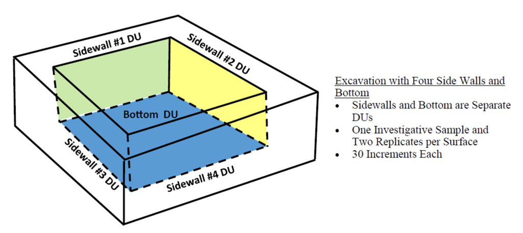
Source: ITRC ISM Update Team, 2020.
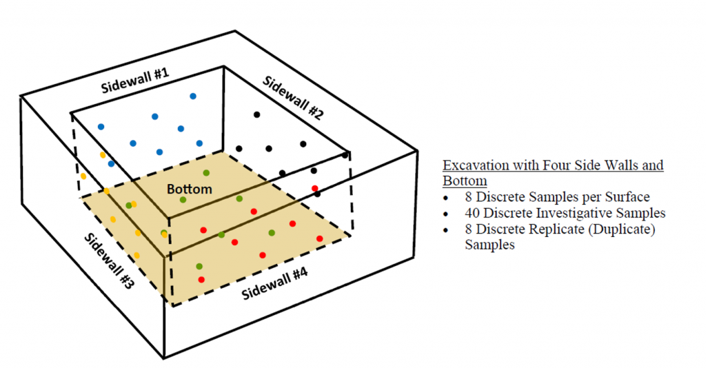
Source: ITRC ISM Update Team, 2020.
A total of five DUs were selected, each with three replicate ISM samples (Figure 3-31), with a total of 30 sample increments collected for each sample. Alternative, discrete sample methods include a total of eight samples from each sidewall and from the bottom of the excavation for a total of 40 investigative samples and eight additional samples collected as duplicates (Figure 3-32). A total of 48 discrete samples are required to be statistically comparative with ISM and account for soil and contaminant heterogeneity.
Using the cost comparison calculator presented in Section 3.4.1.1 the field and laboratory costs are estimated as in Table 3-10.
Table 3-10. Cost estimate for field and laboratory costs for ISM verses discrete sampling for a remediation excavation.
Source: ITRC ISM Update Team, 2020.
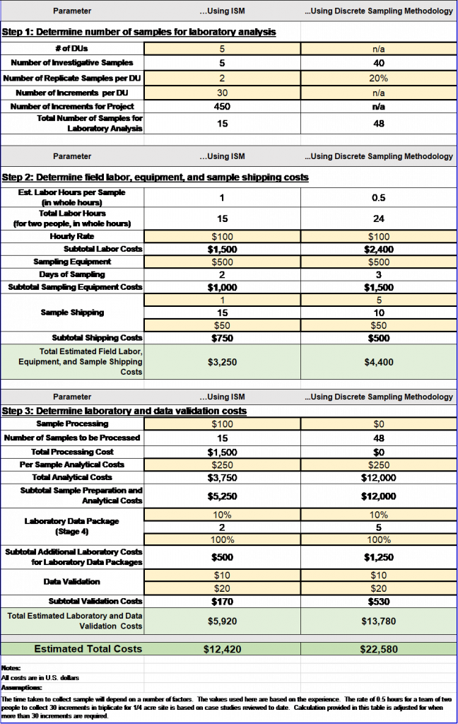
For this example, costs for ISM are much lower than the costs of discrete sampling, and the data used to make decisions are less likely to mis-characterize remaining contamination and lower the potential for remobilization and continued excavation and soil treatment.
3.4.2.4 Classification for waste deposition
ISM can provide a more defensible method for waste characterization by reducing the sampling errors associated with stockpile sampling based on discrete or traditional composite sampling methods. Composite sampling in the sense of combining multiple samples (or, more specifically, increments) from a single DU volume is an improvement over discrete sampling methods and is an approved method for waste characterization. However, ISM provides a more structured approach and ensures both that final bulk samples are prepared by combining waste from a minimum number of points and that the final mass of the sample meets minimum requirements under sampling theory. ISM will reduce the risk that the soil is mis-classified and either denied at the door of a facility or sent as hazardous material when it may have been classified as non-hazardous.
Example 4: stockpile sampling from agricultural field soil. In this example (Figure 3-33 and Figure 3-34), stockpile soil originating from a former agricultural field will be used as fill for the development of a commercial property. It is assumed that arsenic-based pesticides were applied to the agricultural field uniformly with limited mobility and degradation. A stockpile volume of approximately 20,000 ft3 (800 yds3) is assumed and equates to the approximate volume of soil to cover a 1-acre site at a 6-in depth. It is also assumed that the existing stockpile can be flattened or spread out sufficiently so that the interior of the pile can be accessed with a hand sampling device.
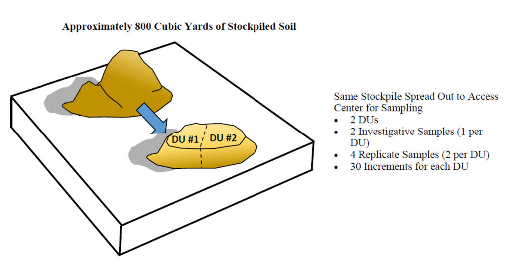
Source: ITRC ISM Update Team, 2020.
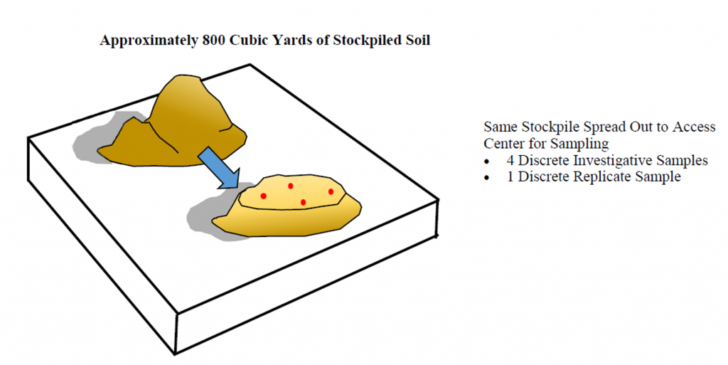
Source: ITRC ISM Update Team, 2020.
Using ISM, one DU per 400 yds3 is recommended as the default exposure area based on the “Guidance for Soil Stockpile Characterization and Evaluation of Imported and Exported Fill Material” (HDOH 2017a). For this example (Figure 3-33), two DUs are required for 800 yds3 of soil. Arsenic-based pesticides are generally water soluble, allowing homogeneous application, so 30 increments were selected to demonstrate representativeness.
The California Department of Toxic Substances guidance, “Information Advisory, Clean Imported Fill Material” (DTSC 2001), provides a table recommending the number of soil samples for a range of soil volumes. This table was used to determine the number of discrete soil samples to be collected from the stockpile (four soil samples), along with the required laboratory analysis (pesticides and metals; Figure 3-34). The collection of background samples for metals are not included in the cost analysis. Using the comparison cost calculator presented in Section 3.4.1.1, the field and laboratory costs are estimated as in Table 3-11.
Table 3-11. Cost estimate for field and laboratory costs for ISM verses discrete sampling of stockpile from agricultural field.
Source: ITRC ISM Update Team, 2020.
In this example, the costs for ISM are approximately twice the costs for discrete sampling. However, the four ISM samples combine soil from 200 points within the stockpile (assuming 30-increment samples), versus four for the discrete samples, and represent a far greater total mass (4 kg to 8 kg versus <1 kg for discrete samples) and were strictly processed at the laboratory to ensure that the data generated were representative of the samples provided (not required for discrete samples). The resulting data are well worth the additional costs and effort, especially if the soil is to be reused in areas where regular exposure could occur.

